Aircraft and Satellite Echoes from TV
transmitters at VHF and UHF
©Ian Roberts, ZS6BTE.
The investigation discussed
below is aimed at detecting aircraft and low altitude satellites using the South
African Broadcasting Corporation’s VHF and UHF TV transmitters. These high
power transmitters (EIRP around 162 kW) are scattered around the country on VHF
and UHF and appear ideal for illuminating aircraft and satellites.
See Table 1 below for reference regarding the transmitters used.
TV Transmitter Exact Frequency Control
To reduce mutual interference
to the TV screens of viewers, the SABC has the various TXs at offsets of a
nominal -26.025 (20m) or +26.025 kHz (20p) from the
“0” offset channel centre frequency. This is further refined into a “precision
offset” regime where the TXs are again offset under experimentation to reduce
this interference to a minimum. For example the Kimberly ch
4 TX on 20m is not at 175250000-26025 Hz (=175,223,975 Hz) but at 175223996 Hz (or
+21 Hz) from the nominal offset of 20m.
All the VHF TXs at the 20m
offset are set to this precision offset under rubidium oscillator control. From
my home I can only confirm the strongest of these TXs, the rest are masked on
the exact frequency.
However, by examining
aircraft reflections from these unseen “partner” TXs, one should be able to
confirm they are on these frequencies. This is because the aircraft reflections
should show simultaneous positive and negative Doppler shifts on the TX carrier
frequency, and its 50 Hz sidebands if powerful enough.
Most of the high power VHF TXs in
The rubidium oscillator
controlled precision offset frequencies for Band 3 ch 4 (20m, “0”, 20p) are in Table
1 below (these are my measurements off-air on long tropospheric scatter paths
using a precision oscillator as reference – they are not official frequencies).
|
Ch |
Site, frequency offset, direction and distance (20M = -26.025 kHz; 20P = +26.025 kHz) |
Polarisation |
Service, Frequency and Date measured |
|
|
4 175.250 |
Potgietersrus 20p Welverdiend 0 Queenstown 0 Beaufort West 20p Oudtshoorn 0 Van Rhynsdorp 0 Villiersdorp 20p |
30°/245km 260°/84km 181°/760 km 195°/902km 190°/634 km 147°/492km 223°/428km 216°/864km 212°/1003km 233°/1097km 221°/1192km distant low power |
H H H H H H H H H H H V |
TV2 175.276089.5 TV1 175.250093.3 TV3 co-channel 20m TV1 co-channel 20p TV1 co-channel “0” TV2 co-channel 20p TV2 175.223996.0 MNET co-channel
20p TV3 co-channel “0” TV1 co-channel “0” MNET co-channel
20p TV1 |
Table 1: Frequency allocations on VHF channel 4.
Directions and distances from Randburg. Reference
TXs, dates and frequencies in red
Tropospheric Scatter
Radio frequencies propagate
further than the visible horizon, typically to k4/3 radius of the earth (i.e.
1.3x), Figure 1. In
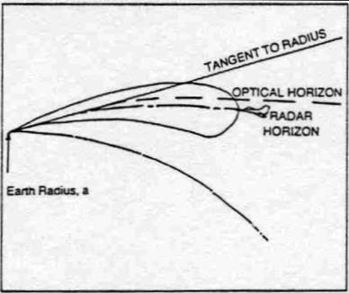
Figure 1: Bending of radio beam due to
refraction (a = true Earth’s radius)
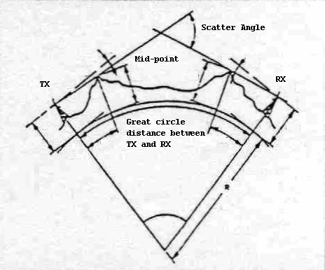
Figure 2: Tropospheric Scatter Path
Geometry
In Figure 2 the zero elevation lines between the TX and RX intersect
and form the Scatter Angle. The smaller the better. Each additional 1 degree in the
scatter angle increases the already high path loss due to the obstructed path
by another 10 dB. In professional practice this is kept below 4 degrees if
possible.
The “volume” around the
intersect point is referred to as the “scatter
volume”. The properties of the scatter volume have an enormous effect on
the quality of the tropo scatter path. Typical height
of the scatter volume is listed in Table
2.
|
Distance,
km |
Height of
Scatter Volume, m agl Favourable
vs. unfavourable paths |
|
150 |
300-2000 |
|
300 |
600-3000 |
|
600 |
3000-20000 |
Table 2: Height of the scatter volume,
meters above smooth ground level
Detection of Aircraft and Satellites
To better understand how all
this fits into the detection of aircraft and satellites refer to Figure 4: Detection Geometry.
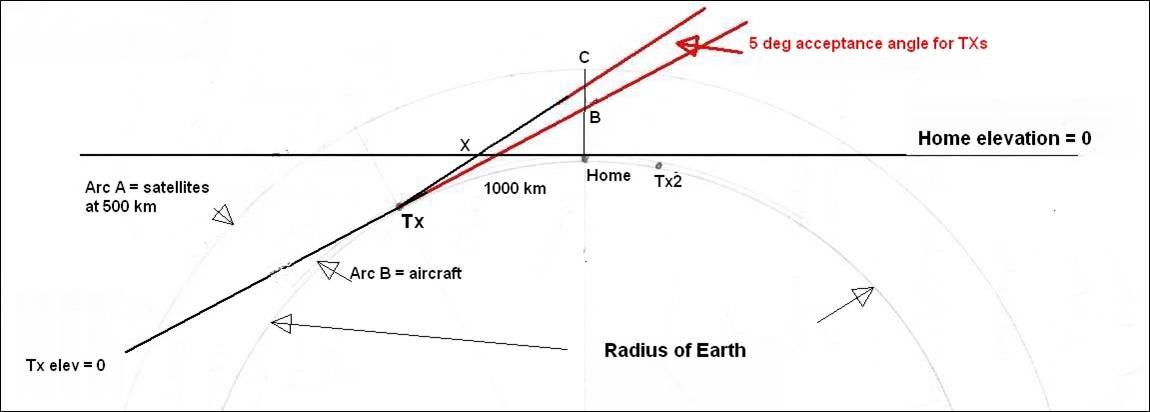
Figure 4: Detection Geometry – side view
Here a similar situation
exists. X is the scatter angle with
associated scatter volume, while TX
and Home represent the TX and RX
sites separated in the scale drawing by 1000 km. Two arcs need to be discussed:
ARC A at 500 km is optimistically
taken as the satellite height above ground – there are relatively few
satellites this low – fortunately the huge International Space Station complex
is at 350 km above ground.
ARC B represents
the maximum height of aircraft, around 35000ft (10.7 km).
Suitable TV Channel to Use, Receiving System
Requirements
VHF is advised because of the
RF advantages.
A TV channel occupied locally
cannot be used due to in-channel noise and there is likely to be a high-power
It follows those scanner-type
receivers with wide front ends cannot be used as they will overload, as will an
unfiltered preamplifier. The wanted signal level is barely above 0 micro volts
into 50 ohms….
The required dynamic range
can be as high as 95-100 dB depending on distance to the local
The ambient RF noise level is
extremely high, as in all city localities with high power, in-band TV
transmitters and computer hash. The receiving system’s noise temperature can be
several hundred or even several thousand Kelvin; preamps at the antenna might
help provided they are filtered and are not driven into gain compression by excessive
input levels.
I used an ICOM IC-R8500, on
VHF a home-brew log periodic antenna with 11.5 dBi of gain on TV ch 4, and low loss cable, no preamp. This setup allows
continual detection of the weak
Signal Processing
The sound card based
Spectrumlab software was used in waterfall mode and an FFT of 262k at a sound
card sampling rate of 44.1 kHz. This reduces the noise floor by nearly 30 dB
compared to “straight” analogue detection. This is a colossal improvement in
receiving system performance. However, the sound card/sound chip should be able
to maintain reasonable performance over a dynamic range of about 70-80 dB when
the input volume is set correctly. If not, severe over-modulation of the
waterfall trace will result, causing false screen image effects.
Questions to Answer, Facts to Confirm, Assorted
Information
1.
An important question
is: can an observer at Home detect aircraft above TX, the TV transmitter, in
Figure 4? The answer is “no”, see point
1 Observed Data below.
2.
Conversely, can
an observer at Home detect aircraft above Home using the TX radio beam? The
answer is “yes”; see point 2 Observed
Data below. In Table 2, the scatter
volume heights available to amateurs are the unfavourable values as amateurs
are unable to utilize mountain tops for TX and Home and will typically have
obstructions to the horizon a few km away, increasing the required scatter
angle and height above ground at X.
3.
It follows
therefore that aircraft at X, even on a shorter path of 600 km for example,
have to be at the maximum height of X above ground to reflect the signal from
TX to Home.
4.
Thus, it seems
that in Figure 4, aircraft within a couple of hundred km
from Home in the direction of TX (Table
2: Height of Scatter volume at ~300 km = 3000m; easily in aircraft cruising
height), should produce strong echoes at home.
5.
While over the
rest of the path TX - Home, particularly the central bit below X, there will be
aircraft echoes if aircraft are in the scatter volume, producing considerable
enhancement.
6.
Occasionally tropospheric ducting will occur; this is an
enhancement mode which will open the entire path, up to thousands of
kilometers, enabling aircraft reflections over that distance, providing the tropo duct is high enough above ground level.. However, it will have no effect on the detection of satellites
other than possibly attenuating the TX beam in the far field by bending the
beam along the earth at low altitude and making satellites more remote.
7.
Regarding
satellite detection, how much power do TV TXs put over the horizon? They have
around 13 dBi gain and a vertical beam width of only
a couple of degrees – does enough power go over the horizon to illuminate
satellites at low elevations?
Observed Data
1.
Using the
2.
However, distant
TXs (428 km), well over the horizon and propagating by tropo
scatter, produce strong echoes on overhead aircraft where the just detectable TV
carrier is enhanced by as much as 20 dB. Confirmed in this case by visual observation
of these aircraft – they are flying over my house (explanation: the scatter
angle is reduced due to the aircraft’s height above ground).
3.
A TX 84 km away
(Welverdiend to the s/w) on the “0” offset produces a display of aircraft
reflections showing Doppler shifts, Figure
5. There are no visible responses from the further afield TXs on the “0”
offset listed in Table 1 – the distances are just too great. In Figure 5, the stronger trace going to
the left is a negative Doppler shift indicating the bistatic range in the
Johannesburg area using the near by Welverdiend TX is increasing, while the
Queenstown TX produces no visible Doppler shift on these aircraft. More on
bistatic range later.
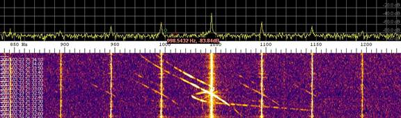
Figure 5: Aircraft echoes received using
the Welverdiend and Queenstown TV TXs. TV carrier frequency in centre, with 50
Hz symmetrical sidebands each side
4.
The Kimberley ch 4 20m offset TX, 428 km s/w, produces a number of
aircraft reflections if these aircraft are on the direct line of sight path Rx
- Tx, while the only other TX on that offset, East
London 760 km s/e, cannot be detected and produces no echoes: Figure 6.
5.
Detection of
aircraft using a UHF high gain antenna array and masthead preamplifier produces
similar aircraft detection as when using VHF TXs, a low gain antenna and no
preamp.
6.
Aircraft flying
directly along the line of sight between the TX and RX produce little or no
Doppler shift.
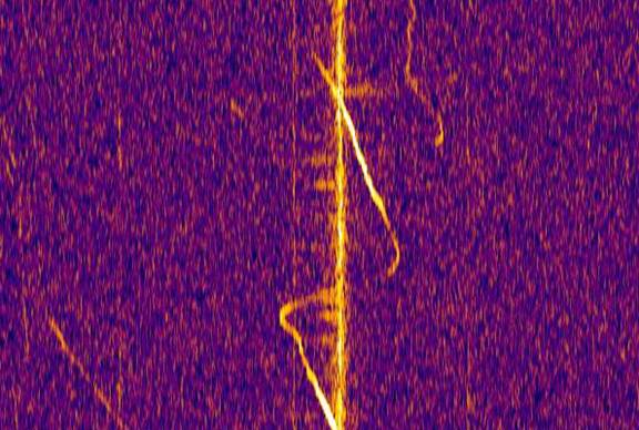
Figure 6: Local aircraft echoes, above
QTH near
More on Path Geometry
Using these results, it is
apparent that aircraft can be detected to a typical range of about 200-400 km if
all the possibilities of a tropospheric scatter path are used. Continual traces
of 15 minutes, corresponding to a distance of 150-200 km for aircraft traveling
around 600-800 km/h, are common on
waterfall displays such as Figures 5 and 6.
This implies that aircraft
within 150 km of Home (see Figure 4)
may be tracked, but possibly not over the central portion of the path in the
scatter volume which may be above aircraft height. In this case, on the probable
maximum 650 km path there may be no reflection from aircraft beneath the
central 350 km or so portion centered under X depending on the altitude of this volume at X.
But all this is over
obstructed paths where the path loss is high.
What about satellites?
Bistatic Doppler Shift on Satellites
We have already established
there is a null pattern above a TV transmitter due to good suppression of any
vertical radiation from the array. In Figure
4 there will be no satellite detection along the line Home – X to the
satellite arc as that line of sight does not intersect ARC A, the satellite
orbital arc above ground, until the far side of the TX at around 1500 km from
Home. In any case the elevation angle from TX to the satellite arc discounts
all possibility of an echo from satellites in the vicinity of TX.
Therefore the only
alternative is above Home along the sight line Home-BC approximately, keeping
the possibility within the red zone. This provides also the best suppression of
unwanted aircraft echoes which could cause confusion of the observed result.
Note that this possible sight-line forms an ellipse around Home.
The detection of satellites
(and aircraft) using this bistatic, passive “radar” technique, is highly
dependent on the Radar Cross Section
of these objects. Too high a frequency (UHF or SHF) used on a satellite complex
such as the ISS, with all its
modules joined to the main body in all directions, causes a reduction in effective
RCS due to the shorter wavelength passing through the gaps without being
reflected. A lower VHF frequency is ideal as the longer wavelength will cause
the beam to be reflected back, i.e. the RCS is more efficiently used.
Satellites, as for aircraft, produce a Doppler shift.
Result of Satellite tracking using TV Transmitters
The calculated Doppler shift
is high for an object such as the ISS, around 14 kHz peak-to-peak
due to the high velocity of 27700 km/h at low range. This is troublesome when
using a SSB bandwidth of 2.5 kHz, offset by some 2-3 kHz to obtain a convenient
beat frequency around 1 kHz at the minimum Doppler shift point. Is there enough
power to detect reflections from a target such as the ISS over a typical
straight-line distance of 1100-1500 km? See the Appendix for a signal-to-noise
ratio calculation.
After a few attempts at
detecting echoes from the ISS at its 350 km altitude under very favourable conditions using various transmitters on ch 4 scattered around
The ISS as a reflective body
at high VHF might have a lower RCS than a typical jet liner. This may be
explained by the numerous flat solar panels, playing such as important part in
visual observation of the ISS and making up a large portion of its apparent
RCS, having little role in reflecting RF, much as the flat panels on stealth
aircraft do not typically reflect radar signals back to the radar receiver.
These solar panels might function effectively as anti-reflection screens. On
the other hand, should they line up briefly the RCS will be very large. The
idea is to capture these brief moments.
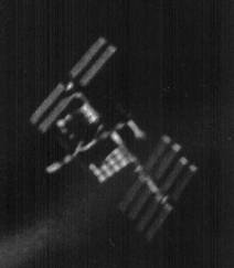
Figure 7: The ISS seen through an
amateur’s telescope – take away those screening solar panels and there’s not
much left….
Are these echoes from the ISS?
After an orbital prediction,
equipment was set up to receive the ISS. Unfortunately nothing was received presumably
due to the horizon cut-off pattern of the TV antenna beams – I was informed by
a former colleague at the SABC that these beams have a vertical beam width of
only a couple of degrees and are aimed at an angle of around -1 degrees to the
horizon.
General Conclusions
1.
While conducting
these experiments various persons in the
2.
Distant aircraft
(~150 km or so) or local aircraft, when crossing the direct line between TX and
RX, enhance the received TX signal by 20 dB or more for a period lasting
possibly some minutes - the more distant, the longer the enhancement in time.
3.
The bistatic Doppler shift from aircraft wobbling around by
only a few meters readily shows up on a recording waterfall – the technique is
very sensitive.
4.
At times the
signals are enormous or extremely weak and will test the dynamic range of the
best receivers.
5.
Aligning TV broadcast
antennas at a negative angle of around -1.5 to -2.0 degrees to the horizon is
almost certainly international practice – it would not make sense to aim at the
horizon as half the EIRP would disappear uselessly into space. This makes
satellite detection using TV broadcast TXs as illuminating sources unlikely if
not impossible as the ERP at an angle of 3-5 degrees or so is likely to be
around 15-20 dB down .
6.
In Figure 5 as the aircraft cross the
carrier frequency where the Doppler shift equals zero, considerable enhancement
of the path’s signal level occurs and echoes from the 50 Hz sidebands become
visible. This corresponds to an enhancement in signal level of at least 25 dB
as the first sidebands in a properly modulated TV transmitter are around 25 or
more dB down on the carrier level.
Appendix – calculations
S/N of a satellite echo
The signal to noise ratio for the predicted total bistatic path to the
ISS may be calculated to check the feasibility of the link, note the
pessimistic RCS of 50 sq m indicating dimensions of only approximately 7 x 7 m –
it might be larger than this. Note also
the calculation assumes the antenna pattern is centered on the horizon, we now
know it is not and the SNR will have a large negative value:
s/n = PTGTGRt0λ2σFTFR
/ (4π)3 kTSRT2
RR2
Pt = Transmitter power, W (10,000)
Gt = Transmit antenna gain as a factor (19.9)
Gr
= Receive antenna gain as a
factor (14.1)
t0 = integration
time in signal processing (FFT 262k “window time”), (5.9 s)
λ = wavelength, m (1.71m~175.25 MHz)
σ = Radar Cross Sectional area, sq m (50sq m)
FT = Transmit antenna to medium
coupling factor, for yagis 0.75
FR = Receive antenna to
medium coupling factor, for yagis 0.75
π = 3.41
k = 1.38 x 10⁻²³ Boltzman’ s constant
TS = System noise temperature (2790 Kelvin), see below
RT = Transmitter
to target distance (1100000m)
RR = Receiver
to target distance (1100000m)
s/n = (10000)(19.9)(14.1)(5.9)(1.71)2(50)(.75)(.75)
/
(4x3.41)3 (1.38 x 10⁻²³ )(2790)(1100000)2 (1100000)2
= 1361472748/143053056
= 9.51
= 9.78
dB, this is ample to detect an echo
RT and RR of some 1500 km (they
are not normally equal as used in this calculation) are necessary to keep the
elevation angle from the TX below 3-5 degrees if possible; otherwise the ISS
will not be illuminated.
RTX
= Transmitter to target
range, meters.
RRX =
Receiver to target range, meters.
L = Distance between TX and RX, meters
Bistatic range = RTX RRX
– L
Around the ellipse
bistatic range does not change, or when the target moves along L, so bistatic
Doppler shift = 0.
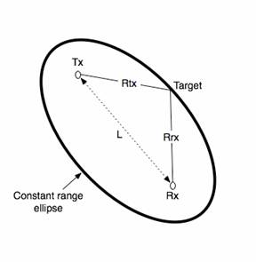
Figure 8: Parameters of
Source: WWW. Wikipedia.com
Bistatic Doppler calculation
Bistatic
Doppler shift is proportional to the rate of change of bistatic range in period
“t1-t” seconds.
Thus,
two bistatic ranges are calculated, firstly at time “t”, then at time “t1”
seconds.
During
this time period the target has moved and increased or decreased the bistatic
range.
The
two values are subtracted to provide the change in bistatic range as at time t1.
Change
in bistatic range ΔR = (RTX RRX – L) – (RTX
RRX – L)1
If
the range has increased the Doppler shift will be negative, and positive if the
range has decreased. The shift can be negative, even if the target is moving
closer to RX.
Bistatic Doppler shift,
Hz f = 1/λ. d/dt. (ΔR)
The
Bistatic Doppler shift in period t+t1 seconds can be read off a
waterfall display as captured in Figure
5 where a RF frequency of 175.25
MHz (λ=1.71m) was used.
The
change in bistatic range can be isolated as:
ΔR, m = f/1. λ/1.
(t1-t)
Thus
in Figure 5, the target causing the
negative 50 Hz Doppler shift in time 22:57:35 – 22:55:45 (approximately 110
seconds as read off), has changed the bistatic range by:
(50s)(1.71m)(110s) = 9404m or an average
speed of 85.5m/s, 308 km/h
Bistatic Doppler shift using multiple TV transmitters locked
onto a common frequency (there will be two bistatic Doppler shifts in this
case) can be read off directly and direction, velocity and distance calculated.
This has not been documented here.
Tropospheric Path Calculations
These
calculations will provide an indication of the signal to be expected from a
distant VHF or UHF transmitter. A tropospheric
scatter path will provide a nearly constant signal around the calculated value.
The steps to follow are:
1. Scatter
angle
2. Path
loss
3. System
noise temperature
4. Signal
to noise ratio
Tropospheric Scatter Angle
The
R = 4/3 earth radius (8446 km)
d = great circle path distance 428 km
h1
and h2 =
respective antenna heights above sea
level, 1.65 and1.385 km
h11
and h12 = height
of radio horizons above sea level, 2 and 1.235 km
d1 and d2 = great circle distance between radio
horizons and respective
antennas, 5 and 100 km
scatter angle θ = θ0 - θ1 –
θ2 radians,
where:
θ0 = d/R
θ1 = h1 -
h11/ d1 + d1/2R
θ2 = h2 -
h12/
d2 + d2/2R
So
scatter angle =
428/8448 – (1.65-2/5 + 5/16896) – (1.385-1.235/100 + 100/16896)
= 0.050663 – (-0.069704) – (0.007419)
= 0.112948 rad
= 6.5 degrees
Tropospheric Scatter Path Loss
LP
= tropospheric scatter path loss, dB
LFS = free space path loss, 92.4 + 20 log d +20
log fGHz
LS = Normalised all
year scatter loss at NS, 57+10log(θ-1)+10 log(f/0.4)
NS = surface refractivity index, around 300
in
LP = LFS + LS – 0.2(NS –
300) dB
= (92.4+20log428+20log0.17525)+(57+10(6.5-1)+10log(0.17525/0.4)
= (129.9)
+ (112.0) + (-3.58)
=
238.32 dB
System Noise Temperature
Tsys = α(Ta) +
To (1- α) + T1 + Tm /gm-1
where:
α = line
transmission coefficient as a factor, 0.8 for a 1 dB loss
Ta = temperature of transmission line, k, equal to Ta for
uncooled lines
To = ambient temperature, k, typically 290
T1 = temperature of 1st RF amplifier stage, 2500k (NF of RX-no
preamp used)
Tm = temperature
of 2nd RF amplifier stage
gm-1 = gain of stage T1
Since
no masthead preamp was used the noise figure of the Rx is taken and Tm /gm-1
is set to 0.
so Tsys = 0.8(290)
+ 290(1-0.8) +2500
= 2790k
Signal to Noise Ratio
over tropospheric scatter path
SNR =
Gt = gain of Tx antenna, dBi (12)
Gr = gain of Rx antenna, dBi (11.5)
Lp = tropospheric scatter path loss, dB (245.7)
Pn = 10 log(kTB) noise power ratio of Rx (-160.1),
k is Boltzman’s
constant 1.38 x10⁻²³ and
B = 2500 Hz in USB, T = Tsys
So
SNR = 40+12+11.5-238.3-(-160.1)
= -14.7 dB
An
FFT of 262k provides an improvement in SNR of about 30 dB:
So
SNR = 30-14.7
= 15.3 dB
This
is in good agreement with the variable 3-20 dB above noise carrier received from
the
My contact information
![]()