
|
Solar Information
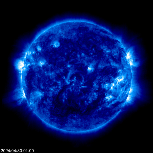
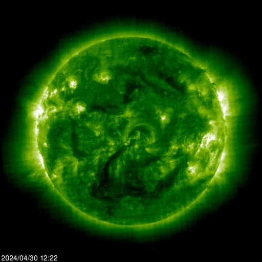
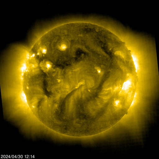
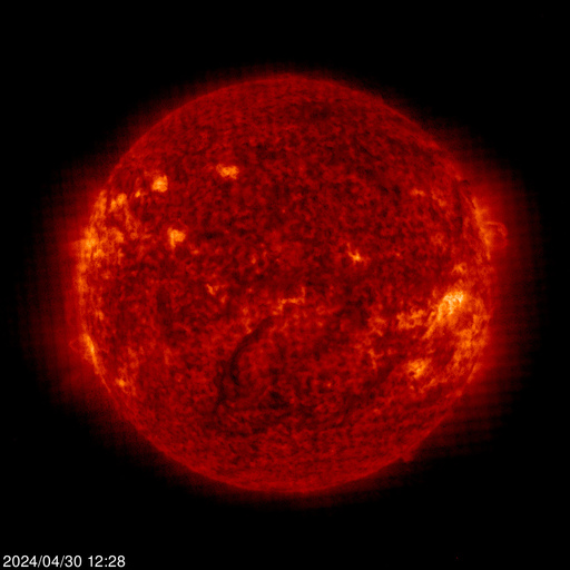
| EIT 171 | EIT 195 | EIT 284 | EIT 304 |
 |
 |
 |
 |
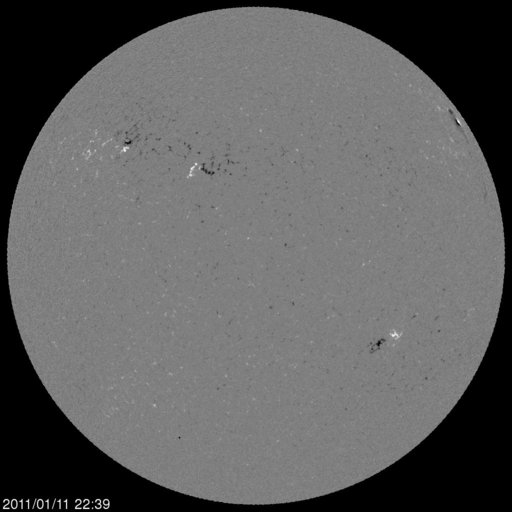
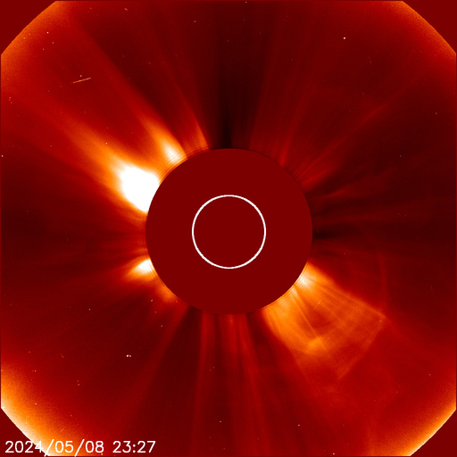
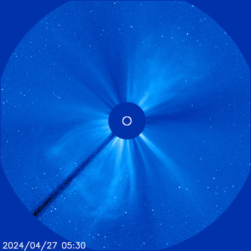
| MDI Continuum | MDI Magnetogram | LASCO C2 | LASCO C3 |
 |
 |
 |
 |
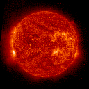
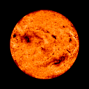
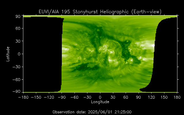
EIT (Extreme ultraviolet Imaging Telescope) images the solar atmosphere at several wavelengths, and therefore, shows solar material at different temperatures. In the images taken at 304 Angstrom the bright material is at 60,000 to 80,000 degrees Kelvin. In those taken at 171 Angstrom, at 1 million degrees. 195 Angstrom images correspond to about 1.5 million Kelvin, 284 Angstrom to 2 million degrees. The hotter the temperature, the higher you look in the solar atmosphere.
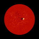
The MDI (Michelson Doppler Imager) images shown here are taken in the continuum near the Ni I 6768 Angstrom line. The most prominent features are the sunspots. This is very much how the Sun looks like in the visible range of the spectrum (for example, looking at it using special 'eclipse' glasses: Remember, do not ever look directly at the Sun!). The magnetogram image shows the magnetic field in the solar photosphere, with black and white indicating opposite polarities.
LASCO (Large Angle Spectrometric Coronagraph) is able to take images of the solar corona by blocking the light coming directly from the Sun with an occulter disk, creating an artificial eclipse within the instrument itself. The position of the solar disk is indicated in the images by the white circle. The most prominent feature of the corona are usually the coronal streamers, those nearly radial bands that can be seen both in C2 and C3. Occasionally, a coronal mass ejection can be seen being expelled away from the Sun and crossing the fields of view of both coronagraphs. The shadow crossing from the lower left corner to the center of the image is the support for the occulter disk. C2 images show the inner solar corona up to 8.4 million kilometers (5.25 million miles) away from the Sun. C3 images have a larger field of view: They encompass 32 diameters of the Sun. To put this in perspective, the diameter of the images is 45 million kilometers (about 30 million miles) at the distance of the Sun, or half of the diameter of the orbit of Mercury. Many bright stars can be seen behind the Sun.
|
|
 |
 |
|
Current solar images Active solar region maps |
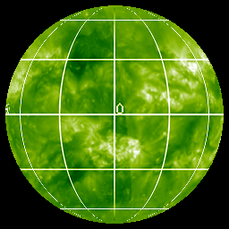 This movie shows a spherical map of the Sun as it currently appears, formed from
a combination of the latest STEREO Ahead and Behind beacon images. The movie
starts with the view of the Sun as seen from Earth, with the 0 degree meridian
line in the middle. The map then rotates through 360 degrees to show the part of
the Sun not visible from Earth. The black wedge shows the part of the Sun not
yet visible to the STEREO spacecraft.
This movie shows a spherical map of the Sun as it currently appears, formed from
a combination of the latest STEREO Ahead and Behind beacon images. The movie
starts with the view of the Sun as seen from Earth, with the 0 degree meridian
line in the middle. The map then rotates through 360 degrees to show the part of
the Sun not visible from Earth. The black wedge shows the part of the Sun not
yet visible to the STEREO spacecraft.


The Total Energy Detector (TED) is an instrument in the Space Environment Monitor (SEM) that has been routinely flown on the NOAA/POES (formerly TIROS) series of polar orbiting meteorological satellites since TIROS-N was launched in November of 1978. The instruments in the SEM, now the second-generation SEM-2, were significantly upgraded beginning with NOAA-15. The upgraded TED, which is designed to monitor the power flux carried into the Earths's atmosphere by precipitating auroral charged particles, now covers particle energies from 50 to 20,000 electron volts (eV) as compared to the earlier TED that extended in energy to only 300 eV.
These measurements are made continually as the satellite passes over the polar aurora regions twice each orbit. Since 1978, observations from almost 300,000 transits over the auroral regions have been gathered under a variety of auroral activity conditions ranging from very quiet to extremely active. Power flux observations accumulated during a single transit over the polar region (which requires about 25 minutes as the satellite moves along its orbit) are used to estimate the total power input by auroral particles to a single polar region. This estimate, which is corrected to take into account how the satellite passes over a statistical auroral oval, is a measure of the level of auroral activity, much as Kp or Ap are measures of magnetic activity. A particle power input of less than 10 gigawatts (10,000,000,000 watts) to a single polar region, either in the North or the South, represents a very low level of auroral activity. A power input of more than 100 gigawatts represents a very high level of Auroral activity. Estimated power inputs as high as 500 gigawatts have been recorded into a single auroral region.
In order to create statistical patterns of auroral power flux, estimated power inputs were computed using observations obtained from more than 100,000 passes over both the northern and southern polar regions. These passes encompassed a wide range of local times and a variety of auroral activity conditions. These polar passes were then sorted into ten auroral activity levels, depending upon the power input estimate. The upper bounds of the first nine levels were defined by a geometric progression of power levels beginning at 2.5 gigawatts up to 96 gigawatts; the tenth level contained estimated power inputs greater than 96 gigawatts. Power flux observations--averaged over one degree of magnetic latitude--from all polar passes with a given activity level were then merged to produce a statistical pattern (a map) of auroral particle power deposition for an entire polar region. Because data were gathered from several satellites, in differing orbits, data were available for almost all local times at latitudes above 45 degrees geomagnetic.
In this fashion ten statistical patterns of auroral particle power input were created, one for each level of auroral activity. The statistical patterns show particle power flux to the atmosphere as a function of magnetic latitude and magnetic local time; coordinates that best order auroral phenomena.
Estimated hemispheric power estimates are computed for each pass over the polar regions as data arrive at the Space Weather Prediction Center from the satellite tracking stations. Once the power input is estimated, the corresponding statistical pattern of auroral power input is selected. Using the Universal Time of the satellite pass, the magnetic latitude and magnetic local time coordinates of the statistical pattern are converted to geographic coordinates; the pattern is then superimposed upon a geographic polar map of either the northern or southern hemisphere.
Normalization factor (n)
A normalization factor of less than 2.0 indicates a reasonable level of
confidence in the estimate of power. The more the value of n exceeds 2.0, the
less confidence should be placed in the estimate of hemispheric power and the
activity level.
The process to estimate the hemispheric power, and the level of auroral activity, involves using this normalization factor which takes into account how effective the satellite was in sampling the aurora during its transit over the polar region. A large (> 2.0) normalization factor indicates that the transit through the aurora was not very effective and the resulting estimate of auroral activity has a lower confidence.


The parameter shown in the upper plot is the effective sunspot number (SSNe) calculated using real-time foF2 observations collected during the 06- or 24-hour period ending at the date/time the SSNe is plotted for. The data plotted in the lower plot are the RMS percent difference between the foF2 observations used in the SSNe calculation and the model foF2 values generated using the SSNe in the URSI-88 foF2 model. The heavy and light curves for both SSNe and the RMS foF2 differences correspond to values calculated using the past 24 hours of foF2 data (heavy lines) and values calculated from the past 06 hours of foF2 data (light lines). Note the quasi-diurnal variation in the 06hr SSNe values, which is due primarily to unequal longitude spacing of the foF2 stations from which the SSNe are being calculated.
The heavy line along the top of the plot is a rough indicator of the number of foF2 values used in the 24hr near-real-time calculation. A wide line indicates that at least 350 values were used, and narrower line indicates less than 350 but more than 200, and no line indicates fewer than 200. The number of foF2 values used and the RMS foF2 difference can be used as an indicator of the usefulness and validity of a particular SSNe value.
The following table summarizes the observations used in calculating the most recent SSNe value. The X entry for a particular station/time indicates there was an foF2 value available and it was used in the SSNe calculation. A - entry indicates that an foF2 value was available, but it was excluded from the SSNe calculation (it was identified as an outlier point). The bar (|) symbol along the time axis of the table indicates the latest-data time (ie., data to the right of this column are from the previous day).
Date: 20091121                          000000000011111111112222
GMLAT  Station              Used  Rej   012345678901234567890123
-----  -------------------  ---- ----  +----|-------------------+
 49.7  Boulder                24   00  |XXXXXXXXXXXXXXXXXXXXXXXX|
 49.4  Fairford               00   00  |    |                   |
 49.1  Chilton                23   00  |XXXXXXXXXXXXXXXXXXXXX XX|
 49.0  Wallops Island         03   00  |    |X       X   X      |
 48.3  Warsaw                 00   00  |    |                   |
 46.8  Dourbes                24   00  |XXXXXXXXXXXXXXXXXXXXXXXX|
 46.3  Pruhonice              00   00  |    |                   |
 43.5  Manzhouli              00   00  |    |                   |
 42.5  Dyess AFB              00   00  |    |                   |
 42.5  Bermuda                00   00  |    |                   |
 42.1  Eglin AFB              00   00  |    |                   |
 41.6  Khabasrovsk            00   00  |    |                   |
 40.6  Point Arguello         00   00  |    |                   |
 38.7  Wakkanai               00   00  |    |                   |
 36.8  Rome                   22   00  |XXXXXXXXXX XXXXXX XXXXXX|
 36.3  Roquetes               20   00  |XXXXXX XXXX XX XX XXXXXX|
 35.4  San Vito               23   00  |XXXXX XXXXXXXXXXXXXXXXXX|
 34.1  Beijing                00   00  |    |                   |
 32.6  Athens                 23   00  |XXXXXXXXXXXXXXXX XXXXXXX|
 32.4  Ashkhabad              02   00  |    |XX                 |
 32.0  El Arenosillo          19   00  |XXXXX    XX XXXXXXXXXXXX|
 30.5  Osan AFB               00   00  |    |                   |
 30.5  Anyang                 00   00  |    |                   |
 30.3  Ramey                  00   00  |    |                   |
 28.7  Kokubunji              00   00  |    |                   |
 22.6  Chongqing              00   00  |    |                   |
 18.9  Okinawa                00   00  |    |                   |
 16.0  Guangzhou              00   00  |    |                   |
  4.0  Kwajalein              20   00  |XXXXXXXXX XX XXXXX  XXXX|
  0.9  Jicamarca              11   06  |-X--|XX    XXXXX  XXX---|
-11.8  Vanimo                 00   00  |    |                   |
-17.0  Ascension Island       00   00  |    |                   |
-18.6  Port Moresby           00   00  |    |                   |
-22.3  Darwin                 20   00  |XXXXXXXXX XXXXX  XXX XXX|
-23.1  Cocos Island           20   01  |XXXXX XXXX- XXXX XXXXXXX|
-25.3  Nuie                   19   00  |XXXX|XXXXX  XX XXXXXXXX |
-28.9  Townsville             22   00  |XXXXXXXX XXXXX XXXXXXXXX|
-32.8  Madimbo                17   00  |    |XXXXXXXXXXXXXXXXX  |
-32.9  Learmonth              00   00  |    |                   |
-36.5  Norfolk Island         22   00  |XX XXXXXXXXXXXXXXXXXXX X|
-36.9  Brisbane               18   00  |XXXXX   XXX   XXXXXXXXXX|
-38.3  Port Stanley           11   00  |X   |     X   XXXXXXXX X|
-38.6  Louisvale              17   00  |    |XXXXXXXXXXXXXXXXX  |
-41.9  Grahamstown            17   00  |    |XXXXXXXXXXXXXXXXX  |
-42.2  Hermanos               17   00  |    |XXXXXXXXXXXXXXXXX  |
-44.7  Camden                 13   00  | XXX|XXXX     X  XX XXX |
-45.1  Mundaring              00   00  |    |                   |
-46.0  Canberra               10   00  |XXXXXX           X  XXX |
-------------------  -----  ---- ----  +----|-------------------+
  # Expected / # Received / Percent: 1128 / 444 /  39.4
The foF2 data used in these calculations were obtained from the NOAA SWPC. These data are being made avaiable from SWPC on a test basis, so there will be occassional periods of data loss as their system is tested.
