 Computer
Assisted Low Profile Antenna Modeling I
Computer
Assisted Low Profile Antenna Modeling I
Using A Personal Computer to Optimize Your Attic Antenna Projects
by Dr. Carol F. Milazzo, KP4MD (posted 13 June 1998)
E-mail: [email protected]
INTRODUCTION
The advent of computer technology has greatly advanced many aspects of
amateur radio. In technical areas such as antenna design, circuit design,
and radio propagation, where one often depended on empirical estimations
and trial and error methods, computer software can often help optimize
results much more reliably. This article describes my experience with applying
this software for low profile antenna modeling.
I was interested in comparing antenna models due to a recent move to
a residential area with restrictive covenants in Omaha, Nebraska. The space
available for the new antennas was inside a peaked roof attic 33 feet above
ground level measuring 32 feet wide, 36 feet long along the north-south
direction, and 8 feet high at the peak. I wanted an antenna for my weekly
schedule between Omaha, Nebraska and New York City. The desirable features
of the antenna were: gain to compensate for the losses due to being located
indoors; broad bandwidth to minimize detuning effects of proximity to the
roof; ability to handle the legal power limit, if necessary; ability to
operate on multiple bands; and, if possible, rejection of signals from
unwanted directions. A computer model offered the convenience of predicting
the performance of different low profile antenna designs prior to physically
building them.
NUMERICAL ELECTROMAGNETICS CODE
|
CONTENTS
|
Many modern antenna analysis programs have their origins in a very large
and complicated FORTRAN program called the Numerical Electromagnetics Code
or "NEC." NEC analyzes wire antennas by dividing them into a number of
segments, calculating the current in each segment and summing the results.
This provides information on the radiation pattern and impedance of the
antenna for any selected frequency. NEC was written in the 1970's and was
composed of tens of thousands of lines of computer code requiring the use
of a mainframe computer inaccessible to most radio amateurs. In 1980, the
team of John Rockway and Jim Logan successfully wrote a very simplified
version called MININEC that had about 500 lines of BASIC and could run
on a personal computer. Since that time, MININEC has evolved through several
versions and enhancements to take advantage of the increased power of modern
personal computers. MININEC provides the basis for a large portion of the
recent amateur radio literature concerning antenna analysis.(1-39)For this
study I obtained the following three freely available demonstration versions
of antenna analysis software:
MININEC
Version 3 can be downloaded at ftp://ftp.funet.fi/pub/ham/antenna/NEC/mininec3.zip
on the Internet. It is also widely available as freeware on many CD-ROMs
and BBS's. It is provided as a BASIC listing and as a compiled BASIC executable
DOS program and can run on any PC compatible computer with an 8080 or later
CPU and at least 512k RAM. Like the original MININEC program, this version
requires the user to work out an antenna model on paper, figure out the
coordinates of the endpoints of each wire, and then enter these numbers
into the program, along with the wire radius and wire connection data.
The input and output consist of text and numerical tables with no graphics.(13)
ELNEC
A demo can be downloaded at ftp://ftp.funet.fi/pub/ham/antenna/elnecdem.exe.
ELNEC is a compiled DOS program that can run on any PC compatible computer
with an 8080 or later CPU, at least 512k RAM and a CGA/EGA/VGA/Hercules
video adapter. This program by Roy Lewallen, W7EL, includes enhancements
to the MININEC3 program allowing a simpler input of information with visual
feedback (3-D graphics of antenna model, radiation pattern plots, graphs
of impedance, VSWR, etc. vs. frequency). The free trial version limits
the number of wire segments to 16 and does not allow printing of graphics
from within the program; however, one can print graphic screens using the
Print Screen key if one first runs the GRAPHICS.EXE program included with
MS-DOS.(25)
NEC4WIN
A free demo of NEC4WIN95 can be downloaded here.
This version requires Microsoft Windows 3.1 or later, or Windows NT or
Windows 95 and a PC compatible computer with a 80386SX or later microprocessor.
This program was written by Madjid Boukri, VE2GMI, and provides a Microsoft
Windows interface to the MININEC3 program, is mouse driven and user friendly.
The Windows graphics are superior to those of the DOS program. The free
evaluation version is fully functional except on one point: you cannot
reload the projects you created and saved. Only "demo" projects files can
be loaded. You can however enter antennas, simulate them, save the projects,
print all diagrams, etc. Projects are saved in ASCII and easily re-entered.
DESIGNING THE MODEL
I selected NEC4WIN as the most appropriate trial program for this project
as the complexity of the antenna models exceeded the limits of the ELNEC
demo program, and the graphic output of NEC4WIN was better suited for this
study. I decided to compare the performance of my previous antenna (a 4-band
crossed inverted vee) with the new proposed antennas. The antenna at my
previous location was a combination of roof mounted inverted vees for 7.1
and 14.1 MHz, and an inverted vee with 60 uH loading inductors 1/4 of the
distance from each end that resonated on both 3.6 MHz and 10.1 MHz. The
feedline was a single 50 ohm coaxial cable. The center support was 34 feet
above ground level with guy wire tie points 11 feet above ground. The main
axis of the antenna was oriented north-south for the main lobes of radiation
to be east and west. Other known data included the lengths of the wires
and guy lines, distances between the tie down points, and average ground
conductivity. Since this antenna had a complicated geometry, figuring the
x, y, and z axis coordinates of the endpoints required using the Pythagorean
Theorem for solving right triangles. I used a spreadsheet table to help
recalculate the coordinates when adjusting wire lengths in the modeling
process. The number of segments affects the accuracy of the calculations.
The length of each segment is generally recommended to be on the order
of .02 wavelengths. A larger number of segments provides greater accuracy,
but this significantly slows the program and requires increasingly larger
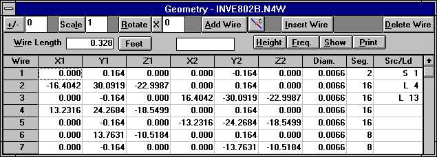
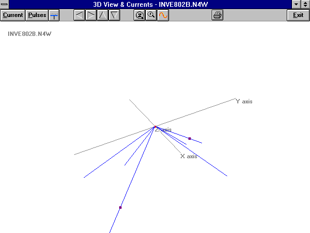
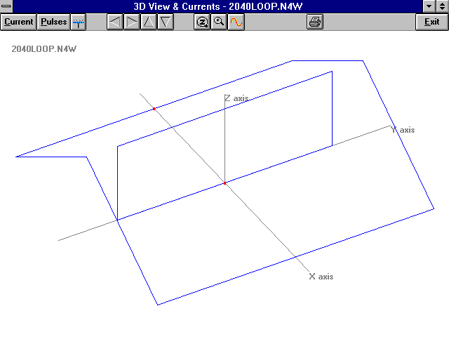
amounts of computer memory. Figure 1 shows the resulting antenna geometry
data for the 4 band crossed inverted vee. Figure 2 shows a 3D view of the
antenna.
|
|
|
Figure 1. Geometry Data of 4 Band Crossed Inverted Vee Antenna
|
Figure 2. 3D View of Crossed Inverted Vee Antenna
|
VALIDATING THE MODEL
An important part of the modeling process is the validation of the model.
This assures the proper geometry and the polarity of each of the wires.
Figure 1 shows the description of each wire with each endpoint with the
greater y coordinate preceding the endpoint with the lesser y coordinate.
This resulted in the proper calculated antenna current pattern. The program
calculated the resonant frequencies of this antenna at 3.6 MHz, 7.0 MHz,
and 10.15 MHz, near the observed resonances of the real antenna. Interestingly,
there was no resonance near 14 MHz. This was also observed in the real
antenna and was probably due to proximity effects between inverted vees
in the particular configuration of this antenna.
ANALYZING THE MODEL
The VOACAP propagation program calculated the ionospheric path for the
Omaha to New York circuit as an azimuth angle of 84.5º and an elevation
angle varying from 12º to 30º depending on season, frequency,
time of day and number of hops. As the best signals were predicted with
a single F2 layer hop at 13º, this elevation was used for model analysis.
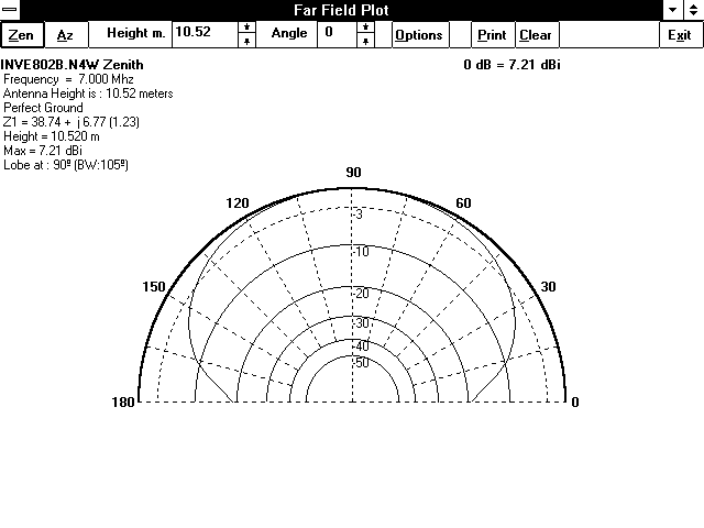
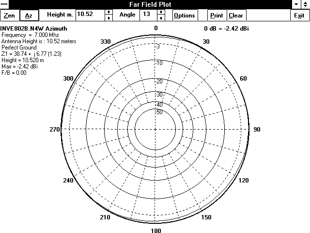
The Miniprop propagation program confirmed these calculated angles. Figures
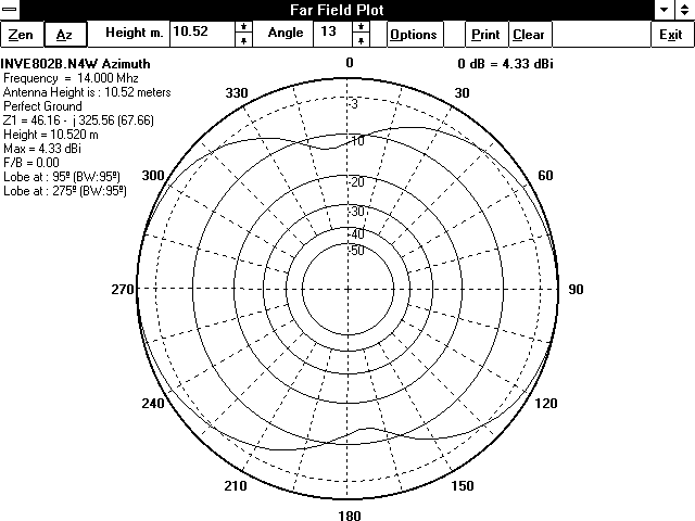
3 to 6 are the radiation patterns for the crossed inverted vees on 7.0
and 14.0 MHz. All azimuth plots were run for an elevation angle of 13º.
The 14.0 MHz radiation patterns show the main lobe at 90º elevation.
According to the modeling convention, 0º on the azimuth pattern represents
the main lobe broadside to the antenna, which in this case would be facing
due east (90º). The direction to New York City would then be 5.5º
counterclockwise from 0º, i.e., at 354.5º on all azimuth radiation
patterns. Figure 8 shows a null (calculated antenna gain of -8.81 dBi),
showing very poor radiation in the desired direction.
|
|
|
Figure 3. Elevation Radiation Pattern for Crossed Inverted Vee
Antenna at 7 MHz
|
Figure 4. Azimuth Radiation Pattern for Crossed Inverted Vee
Antenna at 7 MHz
|

|
|
|
Figure 5. Elevation Radiation Pattern for Crossed Inverted Vee
Antenna at 14 MHz
|
Figure 6. Azimuth Radiation Pattern for Crossed Inverted Vee
Antenna at 14 MHz
|
COMPARING THE MODELS
The first comparison antenna modeled was a variation of a full wave horizontal
loop called the "droopy loop" for 40 meters running along the corners of
the attic, i.e., 36 feet long sides running north and south and a 18 foot
diagonal wire from each of the attic corners up to the peaks on the north
and south ends of the attic.(40) This feedpoint for this loop was at the
center of the 36 foot wire on the east side. The next antenna modeled was
a 20 meter full wave vertical rectangular loop 8 feet high and 28 feet
wide fed at the center of the lower side. The last model was a 20 meter
lazy H consisting of an 8 foot vertical radiator connected to the center
of a 16 foot flat top, and a 36 foot horizontal wire counterpoise. I divided
each loop into 72 equal segments for analysis. The loop design claimed
broad bandwidth and multiple band operation.(14) The vertical loop also
claimed low radiation angle and directionality. The lazy H antenna claimed
omnidirectional low radiation angle.(38) Figures 5 and 6 are views of these
models. The y-axis was oriented north-south; and the x-axis was oriented
east-west. I oriented all directional antennas for maximum radiation in
the east and west directions.
 |
 |
|
Figure 7. 3D View of 40 Meter Droopy Loop and 20 Meter Vertical
Loop Antennas
|
Figure 8. View of 20 Meter Lazy H Antenna
|
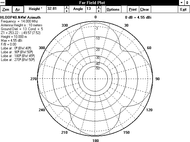
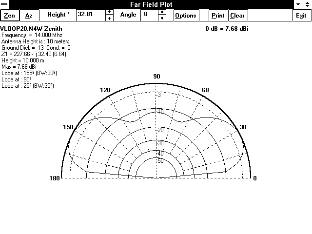
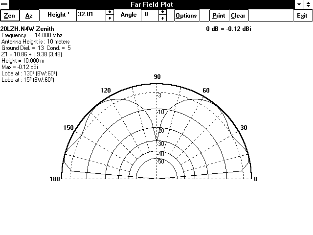
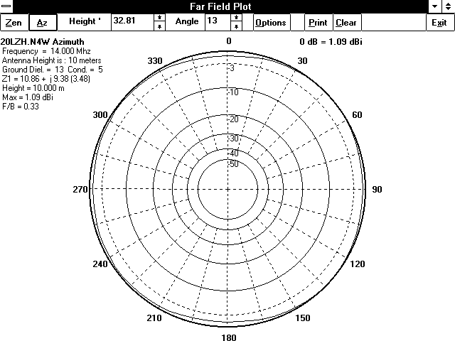
The calculated radiation patterns of these models on 7 MHz and 14 MHz
are in figures 9 to 16.

|
|
|
Figure 9. Elevation Radiation Pattern for 40 Meter Droopy Loop
at 7 MHz
|
Figure 10. Azimuth Radiation Pattern for 40 Meter Droopy Loop
at 7 MHz
|

|
|
|
Figure 11. Elevation Radiation Pattern for 40 Meter Droopy Loop
at 14 MHz
|
Figure 12. Azimuth Radiation Pattern for 40 Meter Droopy Loop
at 14 MHz
|
|

|
|
Figure 13. Elevation Radiation Pattern for 20 Meter Vertical
Loop at 14 MHz
|
Figure 14. Azimuth Radiation Pattern for 20 Meter Vertical Loop
at 14 MHz
|
|
|
|
Figure 15. Elevation Radiation Pattern for 20 Meter Lazy H at
14 MHz
|
Figure 16. Azimuth Radiation Pattern for 20 Meter Lazy H at
14 MHz
|
Here are the calculated elevations of lowest major radiation lobes and
antenna gains for the Omaha to New York circuit for all the modeled antennas:
|
ANTENNA
|
PARAMETER*
|
3.5 MHz
|
7.0 MHz
|
10.0 MHz
|
14.0 MHz
|
18.0 MHz
|
21.0 MHz
|
24.0 MHz
|
28.0 MHz
|
| Crossed inverted vees |
Maj. lobe elev. @ 0º az.
Gain dBi @
13º el. 354º az. |
90º
-4.32 |
90º
-3.22 |
65º
-2.15 |
90º
-8.81 |
20º
+12.67 |
10º
+10.55 |
20º
+13.58 |
35º
+4.12 |
| 40 meter "droopy loop" |
Maj. lobe elev. @ 0º az.
Gain dBi @
13º el. 354º az. |
90º
-2.69 |
85º
-3.41 |
70º
-5.28 |
25º
+3.45 |
25º
+6.17 |
80º
-16.68 |
15º
+5.6 |
15º
-1.12 |
| 20 meter vertical loop |
Maj. lobe elev. @ 0º az.
Gain dBi @
13º el. 354º az. |
90º
-4.99 |
45º
-1.43 |
35º
+1.23 |
25º
+4.95 |
20º
+6.82 |
20º
+6.84 |
15º
+6.54 |
80º
-3.46 |
| 20 meter lazy H |
Maj. lobe elev. @ 0º az.
Gain dBi @
13º el. 354º az. |
25º
-0.50 |
20º
-0.48 |
15º
+0.19 |
15º
-0.08 |
15º
-0.28 |
10º
-0.31 |
10º
-2.33 |
10º
-2.85 |
Table 1. Calculated Parameters for Baseline and
Comparison Antenna Models.
*Parameters are the elevation of first major lobe above the horizon
and the gain in the desired direction.
MININEC may exaggerate gains for antennas lower than 1/4 wavelength
above ground.
Performance of models below antenna design frequencies may be poorer
than calculated due to inefficiencies from high VSWR.
The data for the 7 and 14 MHz were of most relevance as these were the
phone bands on which the best openings were expected during this part of
the sunspot cycle. Compared to the crossed inverted vee antenna, the radiation
pattern of the 40 meter horizontal loop in the desired direction showed
similar gain at 7.0 MHz, increased gain at 14.0 MHz and a somewhat omnidirectional
pattern on all bands. The 20 meter vertical loop showed even greater gain
at 14 MHz with attenuation of signals from the sides. When modeling both
loops together, NEC4WIN calculated negligible induced currents from one
loop to the other, predicting very little interaction as would be expected
due to the loops being in perpendicular planes. The 20 meter lazy H had
the lowest radiation angle but the least gain of all the proposed antennas
at 14 MHz, probably due to it being a shortened radiator as compared to
the full wavelength size of the loops.
COMPARING THE ANTENNAS
I chose to build both the 40 meter and 20 meter loops due to their overall
advantage in gain and bandwidth over the lazy H. I used #14 gauge bare
stranded copper wire for the 20 meter loop. As the 40 meter loop would
run in close proximity to the corners of the attic, I chose insulated #12
gauge stranded copper wire for the that one. Ceramic end insulators tied
to screw eyes supported the low antenna corners. I passed nylon cords through
3/4 inch pulleys in the attic peak to support the ceramic insulators for
the high loop corners. I tied the feedpoint ends of the loops to center-type
ceramic insulators and directly fed them with 90 foot lengths (an electrical
wavelength at 7.2 MHz) of polyethylene dielectric RG-8/U coaxial cable.
The electrical wavelength is equal to the free space wavelength multiplied
by the velocity factor of the transmission line, which is 0.66 in the case
of polyethylene dielectric RG-8/U. I chose this length because transmission
lines measuring an electrical half-wavelength, or multiples thereof, duplicate
the impedance at the load end of the antenna and eliminate the need for
a matching transformer between the feedline and the antenna. A 90 foot
length of transmission line provides this effect at 3.6, 7.2, 10.8, 14.4,
18, 21.6, 25.2, and 28.8 MHz-frequencies in or near several of the amateur
HF bands. I avoided foam dielectric coaxial cable because: 1) it has a
lower voltage rating that might be exceeded by higher VSWR's when using
the legal power limit on the WARC bands; and, 2) the heating of the foam
dielectric with high VSWR's can cause the center conductor to migrate through
the dielectric forming impedance bumps and increasing losses, heating and
possibly shorting the center conductor to the shield. In the event that
your power levels will not exceed 100 watts or so, you should be able to
use RG-58/U or foam dielectric cable, being sure to calculate the cable
lengths using the appropriate velocity factor for your cable if you wish
to use a multiple of an electrical half-wavelength. Open-wire transmission
lines would simplify the feeding and matching of the antennas, but I could
not use these in my indoor installation due to a limited space for threading
the cables from the attic to the station in the basement and due to the
presence of metal heating ducts within that space.
I took the following measurements at the transmitter end of the transmission
lines. The observed resonant frequencies were reasonably close to the calculated
frequencies despite expected differences due to proximity effects of the
attic structures.
|
ANTENNA
|
CALCULATED RESONANT
FREQUENCY (MHz)
|
OBSERVED RESONANT
FREQUENCY (MHz)
|
2:1 VSWR BANDWIDTH
OBSERVED (MHz)
|
|
40 meter "droopy loop"
|
7.12 MHz
|
7.04 MHz
|
0.6 MHz
|
|
20 meter vertical loop
|
14.16 MHz
|
14.00 MHz
|
1.6 MHz
|
Table 2. Calculated and Observed Resonant Frequencies
and Bandwidths of Loop Antennas.
On the air tests using both loops gave good results on scheduled contacts
as NEC4WIN predicted. Either loop could handle either 100 watts or 1 kW
of power; however, a test transmission of 1 kW on 7 MHz using the droopy
loop induced high RF currents in the house wiring, tripping all the ground-fault
current interruptors and triggering the home security system. One should
assure compliance with the latest safety guidelines for RF exposure if
planning to use high power with this type of antenna.(41,42) On some 20
meter schedules, the signal on the vertical loop was consistently ½
to 1 S unit stronger than on the horizontal loop, just as NEC4WIN predicted.
At other times, switching between the 40 meter loop and 20 meter loop gave
an interesting diversity reception effect, with signals at times stronger
by several S units on one antenna or the other. This inconsistent difference
in gain between the loops was probably due to changes in the incident radiation
angle under varying propagation conditions. The loops have given me good
signal reports with contacts to both coasts during openings on all bands
from 40 through 15 meters using an antenna tuner. The antenna tuner also
allowed the use of the 40 meter loop for short skip contacts using 100
watts on 80 meters. It may be difficult to use higher power levels on 80
meters since the half wavelength of transmission line would duplicate the
high impedance of antenna feedpoint at the tuner, producing very high RF
voltages that could exceed the component ratings of the antenna tuner.
CONCLUSION
Computer antenna modeling offers a practical way to save time and effort
in the selection of antennas for the operator's requirements prior to actual
construction. Currently available software makes computer antenna modeling
for antenna projects easily accessible to the average amateur radio operator.
BIBLIOGRAPHY: COMPUTER ANTENNA ANALYSIS
-
"Modeling HF Antennas with MININEC", The ARRL Antenna Compendium,
Vol. 3. [MININEC]
-
"MN Antenna Analysis Software for the IBM PC", QST, Sep. 1988, p.
41. [MN]
-
"K6STI's MN and Yagi Optimizer Antenna Analysis Software",
QST,
Aug. 1990, p. 41. [MN, YO]
-
"MININEC: The Other Edge of The Sword", Lewallen, R, W7EL, QST,
Feb, 1991, p. 18. [MININEC]
-
"Antenna Software - AO 5.0", Beezley, B, K6STI,
QST, Apr. 1993,
p. 45. [AO]
-
"QST Compares Antenna Modeling Software", Straw, D, N6BV, QST, Oct.
1995, p. 72.
-
"The Convoluted Loop", Hart, T, W5QJR, Ham Radio, Apr. 1989, Vol.
22:4, pp. 89-97. [MININEC]
-
"Ham Radio Techniques: The Yagi Optimizer Disk", Orr, W, W6SAI, Ham
Radio, May 1989, Vol. 22:5, p.83. [YO]
-
"Ham Radio Techniques: Antenna Gain", Orr, W, W6SAI,
Ham Radio,
Jan. 1990, Vol. 23:1, pp. 30-31. [MN]
-
"Ham Radio Techniques: The MN Analysis Program (That was then, this is
now)", Orr, W, W6SAI, Ham Radio, Feb. 1990, Vol. 23:2, pp. 34-39.
[MN]
-
"Ham Radio Techniques: 160 Meter Antenna Problems and Solutions", Orr,
W, W6SAI, Ham Radio, Mar. 1990, Vol. 23:3, pp. 49-54. [MN]
-
"Ham Radio Techniques: The Yagi Optimizer", Orr, W, W6SAI, Ham Radio,
Apr. 1990, Vol. 23:4, pp. 68-71. [YO]
-
"Using MININEC for Antenna Analysis: Elements of MININEC theory", Haviland,
RP, W4MB, Communications Quarterly, Nov. 1990, pp. 16-22. [MININEC]
-
"The Quad Antenna: Rectangular and Square Loops: Design and performance
data for any square, rectangular or diamond loop", Haviland, RP, W4MB,
Communications
Quarterly, Vol. 1:1, Spring 1991, pp. 11-22. [MININEC]
-
"Yagi Optimization and Observations on Frequency Offset and Element Taper
Problems: Using computer programs for antenna analysis", Orr, W, W6SAI,
Communications
Quarterly, Vol. 1:1, Spring 1991, pp. 79-85. [MININEC, YO]
-
"Antenna Angle of Radiation Considerations: Performance comparison of Quads
and Yagis mounted at low heights: Part 1", Luetzelschwab, C, K9LA, Communications
Quarterly, Vol 1:3, Summer 1991, pp. 37-42. [MN, YAGINEC]
-
"The Triangle Antenna: An alternative horizontal omnidirectional antenna",
Beesley, B, K6STI, Communications Quarterly, Vol 1:4. Fall 1991,
pp. 49-60. [MN]
-
"Antenna Angle of Radiation Considerations: Performance comparison of Quads
and Yagis mounted at low heights: Part 2", Luetzelschwab, C, K9LA, Communications
Quarterly, Vol 1:4, Fall 1991, pp. 61-67. [MN, YAGINEC]
-
"Antenna Structure Interaction: Modeling with MININEC", Haviland, RP, W4MB,
Communications
Quarterly, Vol 1:4, Fall 1991, pp. 73-78. [MININEC]
-
"The 160 Meter Semi Vertical: A case history", Elwell, H, N4UH, Communications
Quarterly, Vol 2:1, Winter 1992, pp. 81-93. [MININEC]
-
"Parasitic Elements for Pattern Shaping in Vertical Antennas: Enhances
patter control using parasitic elements", Haviland, RP, W4MB, Communications
Quarterly, Vol 2:3, Summer 1992, pp. 28-34. [MININEC]
-
"Supergain Antennas: Possibilities and problems", Haviland, RP, W4MB, Communications
Quarterly, Vol 2:3, Summer 1992, pp. 55-72. [MININEC]
-
"The Effects of Antenna Height on Other Antenna Properties: a computer
study", Cebik, LB, W4RNL, Communications Quarterly, Vol 2:4, Fall
1992, pp. 57-79. [ELNEC]
-
"The Unidirectional Long Wire Antenna: A look at this useful alternative
to the Yagi", Haviland, RP, W4MB, Communications Quarterly, Vol
3:4, Fall 1993, pp.35-41. [MININEC]
-
"Comparing MININECS: A guide to choosing an antenna optimization program",
Cebik, LB, W4RNL, Communications Quarterly, Vol 4:2, Spring 1994,
pp.53-72. [AM, AO, ELNEC]
-
"Modeling and Understanding Small Beams Part 1: The X-beam", Cebik, LB,
W4RNL, Communications Quarterly, Vol 5:1, Winter 1995, pp. 33-50.
[ELNEC]
-
"Source Data Display Program for ELNEC: Use this stand-alone program to
plot or print data using ELNEC files", Cefalo, TV, WA1SPI, Communications
Quarterly, Vol 5:2, Spring 1995, pp. 31-36. [ELNEC]
-
"Modeling and Understanding Small Beams Part 2: VK2ABQ squares and Moxon
rectangles", Cebik, LB, W4RNL, Communications Quarterly, Vol 5:2,
Spring 1995, pp. 55-70. [ELNEC]"
-
"Understanding Elevated Vertical Antennas: Useful information about a popular
antenna type", Shanney, B, KJ6GR, Communications Quarterly, Vol
5:2, Spring 1995, pp. 71-76. [MININEC]
-
"Modeling and Understanding Small Beams Part 3: The EDZ family of antennas",
Cebik, LB, W4RNL, Communications Quarterly, Vol 5:4, Fall 1995,
pp. 53-65. [ELNEC]
-
"Quarterly Review: NEC-WIN Basic for Windows", Cebik, LB, W4RNL, Communications
Quarterly, Vol 6:1, Winter 1996, pp. 55-56. [NEC-WIN]
-
"Quarterly Computing: NEC-WIN Basic for Windows", Thompson, B, AA1IP, Communications
Quarterly, Vol 6:1, Winter 1996, pp. 86-88. [NEC-WIN]
-
"Fractal and Shaped Dipoles: Some simple fractal dipoles, their benefits
and limitations", Cohen, N, N1IR, Communications Quarterly, Vol
6:2, Spring 1996, pp. 25-36. [EZNEC]
-
"Modeling and Understanding Small Beams Part 4: Linear loaded Yagis", Cebik,
LB, W4RNL, Communications Quarterly, Vol 6:3, Summer 1996, pp. 85-106.
[ELNEC]
-
"Modeling and Understanding Small Beams Part 5: The ZL Special", Cebik,
LB, W4RNL, Communications Quarterly, Vol 7:1, Winter 1997, pp. 72-90.
[EZNEC]
-
"Optimal Elevated Radial Vertical Antennas: Design minimizes effects of
unequal radials' currents", Weber, D, K5IU, Communications Quarterly,
Vol 7:2, Spring 1997, pp. 9-27. [NEC-WIN]
-
"EZNEC For DOS: The marriage of ELNEC and NEC-2". Cebik, LB, W4RNL, Communications
Quarterly, Vol 7:2, Spring 1997, pp. 28-30. [ELNEC, EZNEC]
-
"The Lazy H Vertical: A versatile antenna for DX work", Severns, R, N6LF,
Communications
Quarterly, Vol 7:2, Spring 1997, pp. 31-40. [NEC-2]
-
"Modeling and Understanding Small Beams Part 6: Fans, bowties, butterflies,
and dragonflies", Cebik, LB, W4RNL,
Communications Quarterly, Vol
7:2, Spring 1997, pp. 81-97. [ELNEC]
-
"The Droopy Loop", Newton, P, KJ7MZ, QST, Vol 80:7,July 1996, pp.
57-58.
-
"The FCC's New RF-Exposure Regulations", Hare, E, KA1CV, QST, Vol
81:1, January 1997, pp.47-49.
-
"What's New About the FCC's New RF-Exposure Regulations?", Hare, E, W1RFI,
QST,
Vol 81:10, pp.51-52.
APPENDIX: NEC4WIN Antenna Model Files n4wmodel.zip
CM
CM NEC4WIN File
CM 80/40/30/20 meter crossed inverted vees
CM Resonated on 3.575, 7.1, 10.12 and 14.075 MHz
CM 82 segments
CM
CE
GND Reference
UNITS Feet
Height 34.5144
Over Perfect Ground
Circular Boundary
F 7.000
GW 1 2 0.000 0.164 0.000 0.000 -0.164 0.000 0.0066
GW 2 16 -16.4042 30.0919 -22.9987 0.000 0.164 0.000 0.0066
GW 3 16 0.000 -0.164 0.000 16.4042 -30.0919 -22.9987 0.0066
GW 4 16 13.2316 24.2684 -18.5499 0.000 0.164 0.000 0.0066
GW 5 16 0.000 -0.164 0.000 -13.2316 -24.2684 -18.5499 0.0066
GW 6 8 0.000 13.7631 -10.5184 0.000 0.164 0.000 0.0066
GW 7 8 0.000 -0.164 0.000 0.000 -13.7631 -10.5184 0.0066
S 1 1 100 0
LI 1 5 .1 60
LI 2 30 .1 60
Coax 50 |
CM
CM NEC4WIN File
CM 40 meter droopy loop
CM For attic 8' high x 36' long x 32' wide
CM 72 segments
CM
CE
GND Reference
UNITS Feet
Height 32.8101
Over Ground 13 5 (Diel. - Cond. µSiemens)
Circular Boundary
F 7.000
GW 1 18 16.000 -18.000 0.000 16.000 18.000 0.000 0.0069
GW 2 9 16.000 18.000 0.000 0.000 18.000 8.000 0.0069
GW 3 9 0.000 18.000 8.000 -16.000 18.000 0.000 0.0069
GW 4 18 -16.000 18.000 0.000 -16.000 -18.000 0.000 0.0069
GW 5 9 -16.000 -18.000 0.000 0.000 -18.000 8.000 0.0069
GW 6 9 0.000 -18.000 8.000 16.000 -18.000 0.000 0.0069
S 1 9 100 0
Coax 50 |
20 Meter Vertical rectangular loop vloop20.n4w
CM
CM NEC4WIN File
CM 20 meter vertical rectangular loop
CM For attic 8' high x 36' long x 32' wide
CM 72 segments
CM
CE
GND Reference
UNITS Feet
Height 32.8086
Over Ground 13 5 (Diel. - Cond. µSiemens)
Circular Boundary
F 14.000
GW 1 28 0.000 14.000 0.000 0.000 -14.000 0.000 0.0052
GW 2 8 0.000 -14.000 0.000 0.000 -14.000 8.000 0.0052
GW 3 28 0.000 -14.000 8.000 0.000 14.000 8.000 0.0052
GW 4 8 0.000 14.000 8.000 0.000 14.000 0.000 0.0052
S 1 14 100 0
Coax 50 |
CM
CM NEC4WIN File
CM 20 Meter Lazy H Antenna
CM 30 segments
CM
CE
GND Reference
UNITS Feet
Height 32.810
Over Ground 13 5 (Diel. - Cond. µSiemens)
Circular Boundary
F 14.000
GW 1 9 0.000 -18.000 0.000 0.000 0.000 0.000 0.0066
GW 2 9 0.000 18.000 0.000 0.000 0.000 0.000 0.0066
GW 3 4 0.000 0.000 0.000 0.000 0.000 8.000 0.0066
GW 4 4 0.000 0.000 8.000 0.000 -8.000 8.000 0.0066
GW 5 4 0.000 0.000 8.000 0.000 8.000 8.000 0.0066
S 1 18 100 0
Coax 50 |
CAPTIONS
Figure 1. Geometry Data of 4 Band Crossed Inverted Vee Antenna
Figure 2. 3D View of Crossed Inverted Vee Antenna
Figure 3. 3D View of 40 Meter Droopy Loop and 20 Meter Vertical Loop
Antennas
Figure 4. View of 20 Meter Lazy H Antenna
Figure 5. Elevation Radiation Pattern for Crossed Inverted Vee Antenna
at 7 MHz
Figure 6. Azimuth Radiation Pattern for Crossed Inverted Vee Antenna
at 7 MHz
Figure 7. Elevation Radiation Pattern for Crossed Inverted Vee Antenna
at 14 MHz
Figure 8. Azimuth Radiation Pattern for Crossed Inverted Vee Antenna
at 14 MHz
Figure 9. Elevation Radiation Pattern for 40 Meter Droopy Loop at 7
MHz
Figure 10. Azimuth Radiation Pattern for 40 Meter Droopy Loop at 7
MHz
Figure 11 Elevation Radiation Pattern for 40 Meter Droopy Loop at 14
MHz
Figure 12. Azimuth Radiation Pattern for 40 Meter Droopy Loop at 14
MHz
Figure 13 Elevation Radiation Pattern for 20 Meter Vertical Loop at
14 MHz
Figure 14. Azimuth Radiation Pattern for 20 Meter Vertical Loop at
14 MHz
Figure 15 Elevation Radiation Pattern for 20 Meter Lazy H at 14 MHz
Figure 16. Azimuth Radiation Pattern for 20 Meter Lazy H at 14 MHz
Return to KP4MD Home Page