Radio Frequency Ranging

 Multi Carrier Phase Ranging (MCPR) is a technique to estimate the distance between sender and receiver. This project uses two QPSK carriers to selectively transmit data to a specific distance from a sender because the phase changes faster over the distance and time.  

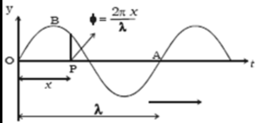
Forumula:   y(x,t) = A sin(kx - 2 pi t )   and, k is the wave number, 2 pi / lambda   and, lambda = c / f

Theory of MCPR phase ranging

Start  with two signals: a carrier- and a reference signal; In the  simulation below, the two carriers are separated by 1.1 (high = 1.1 times low frequency, ie. variable deltafreq). 

 The samplerate (variable fs) is in this simulation 1024 samples/seconds and the speed of the wave (c) is 110 meters/seconds - this is summarized in the table below.

carrier	lambda: 10m	11Hz	c=110m/s
reference	lambda: 11m	10Hz	c=110m/s

 

%matlab / octave script

ref = 10, fs = 1024, c=110, deltafreq=1.1;

carrier=deltafreq*ref;

lambda_ref     =  c / (ref);

lambda_carrier =  c / (carrier);

 

t=0:(1/fs):1.2;

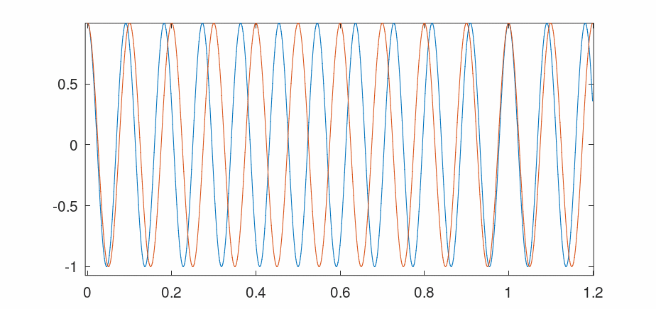
x = cos(carrier * 2*pi*t) + i*sin(carrier * 2*pi*t);

y = cos(ref * 2*pi*(t)) + i*sin(ref * 2*pi*(t));

The phases of both signals (reference and carrier) drift  over time (figure below).  

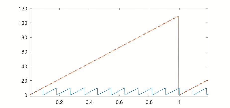
The distance a wave travels came be reconstructed from that phase difference. It  is calculated with the code below: 

xa,ya - the angles of carrier and reference signal

xd,yd - fraction of the distance travelled (lambda = wavelength)

xa = mod(2*pi + angle(x),2*pi);

ya = mod(2*pi+angle(y),2*pi);

xd = lambda_carrier*xa/(2*pi);

yd = lambda_ref*ya/(2*pi);

In the graph, the blue line is the fraction(ie. phase/2pi) of wavelength of the  reference signal, while the red line is the total distance.

To find this total distance after n cycles of the reference signal, the two arrays xd and yd are parameters  of  the ‘Chinese Remainder Theory’ (CRT)  .   The Chinese Remainder Theorem  calculates the least common multiple.

The CRT algorithm    works only  if wavelengths that are relative prime, and, the distances must be integers.  The maximum distance one can measure is 110 meter (that is: 110=10*11, the product of  wavelength of carrier and reference signal)

 

%matlab / octave script

phaseranging = arrayfun( @calcCRT, round(xd), round(yd)  );

function x=calcCRT(a,b)

  d = [10 11];

  rem = [a b];

  Ntot=prod( d );

  sumatotal = 0;

  

  for i = 1:length(rem)

   Ni = Ntot/d(i);

   [ G x ] = gcd(Ni,d(i));

   if G==1

    x = x + d(i);

    

    sumatotal=sumatotal + rem(i)*Ni*x;

   else

     disp(“no inverse")

     break

   endif

   

  endfor

  

  x=mod(sumatotal,Ntot);

end

 

Dual carrier PSK

Dual carrier PKS is a  mode to communicate digital data to a specific distance of the sender. Together with near-field direct antenna modulation, you can also specify the desired angle between the sender and receiver (beam forming).  This concept is used in the puzzle below.. 

Simulation

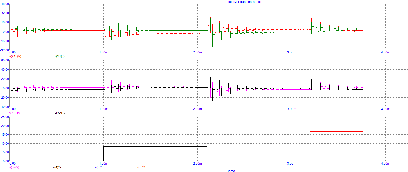
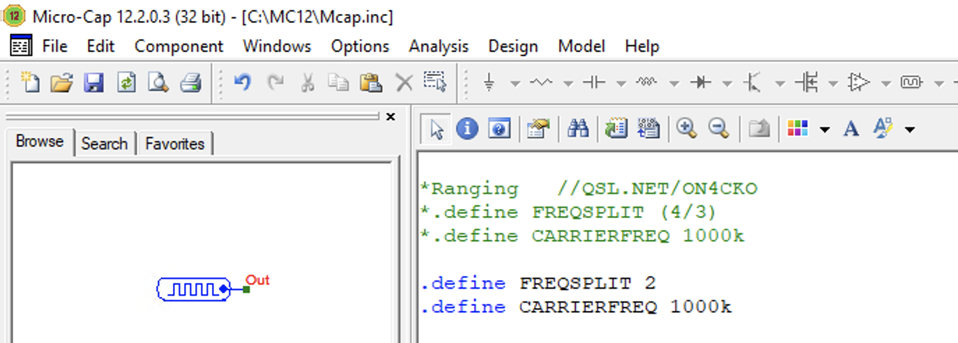
In the simulation below, a 4PSK signal is modulated on two carriers: 1MHz and 500KHz; The signal is sent over a transmission line with parameter TD=0.3333 sec, or, a direct line (TD=0).  The MICROCAP schematic is here - it has some tunable parameters that are discussed below.

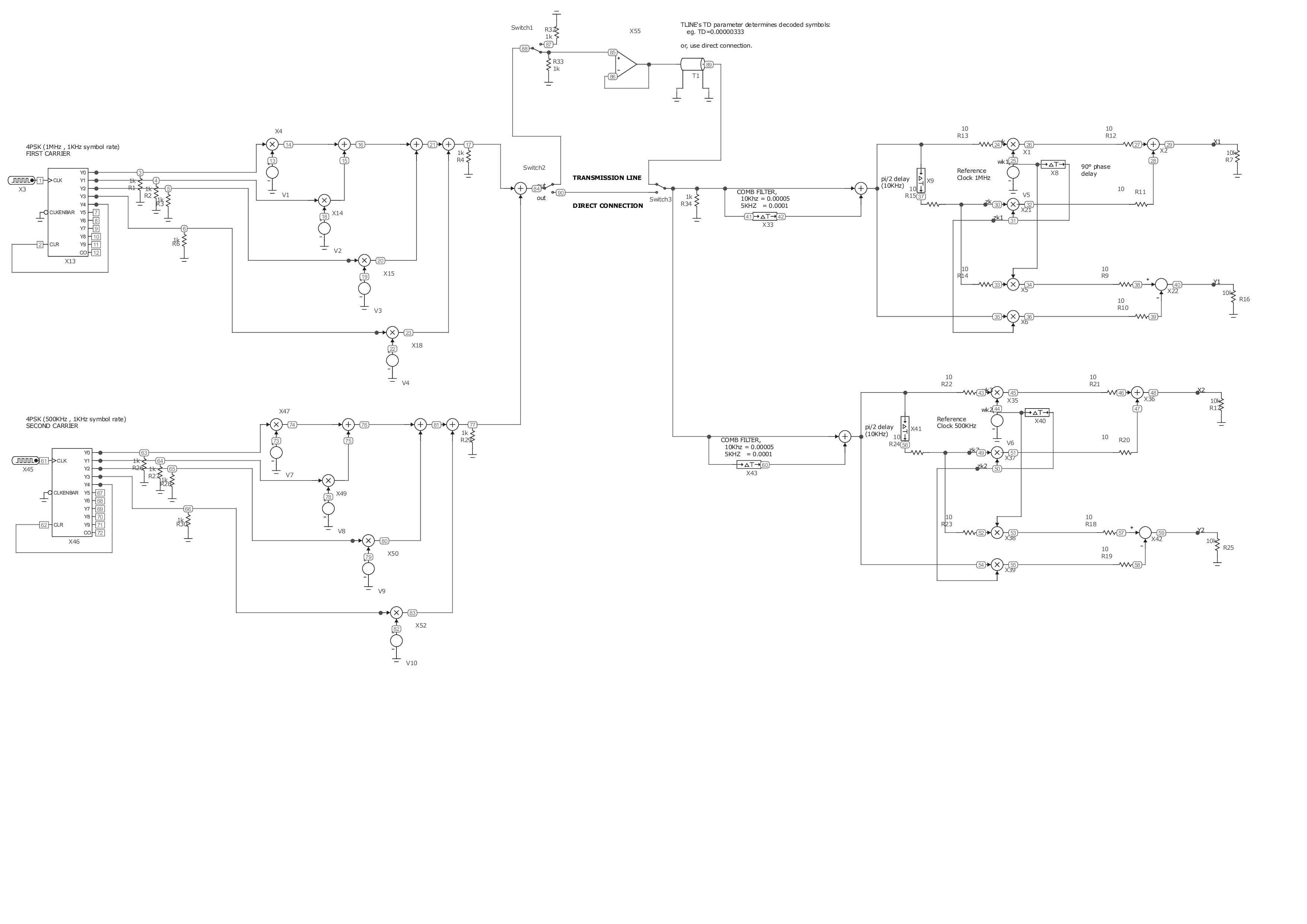
The PSK modulator (in the schematic on the left)  is a   selector of signal sources with phases in four quadrants: 0°, 90°, 180° and 270° (the repeated symbol are shown in the lowest graphs ) for the high and low frequency (currently 1MHz and 500kHz). The settings has to be defined in the Options menu (’User Definitions’).

The symbols are detected after a comb-filter (middle section) to suppress the unwanted carrier. Warning: The comb-filter has some influence on the decoded signals.

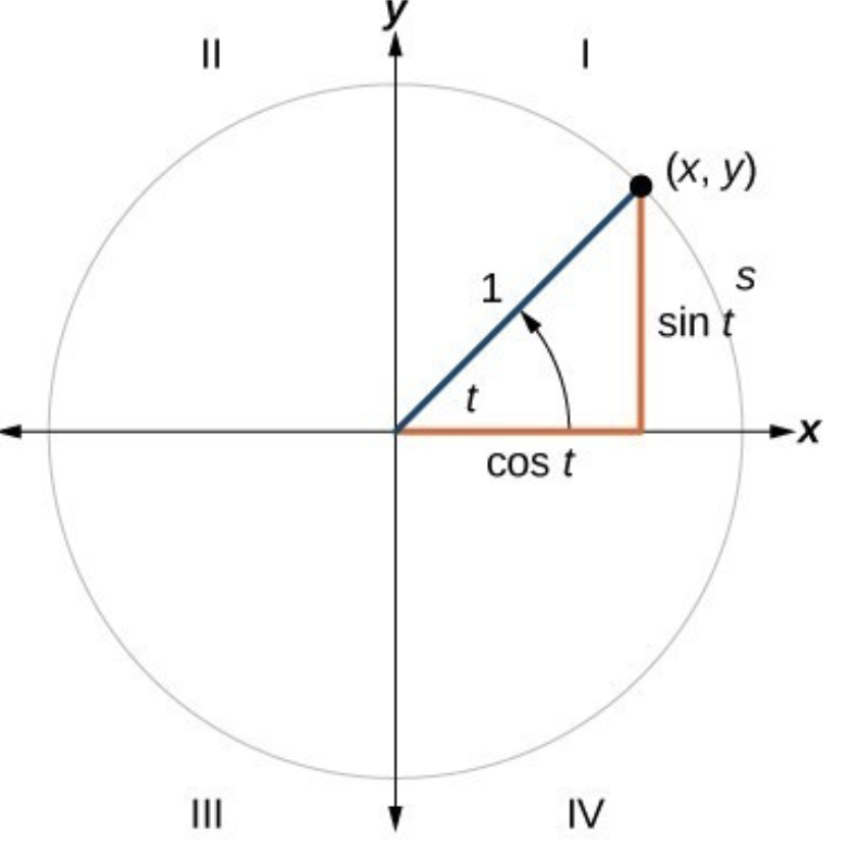
The PSK demodulator has two outputs: x and y (for the high- and low carrier). It is based on the QPSK demodulator from the paper, FPGA Implementation of pi/4-QPSK Modulator and Demodulator: To compare the phase of two signals ‘r’ and ’s’, calculate the following to get the coordinates on the unit circle.

X = cos(s) cos(r) + sin(s) sin(r)        = cos( s - r ) Y = sin(s) cos(r) - cos(s) sin(r)      =  sin( s - r) The symbol (x,y)  defined two  bits i and q:  i=1, if x>0 i=0, if x<0 q=1, if y>0 q=0, if y<0

Receiving dualpsk

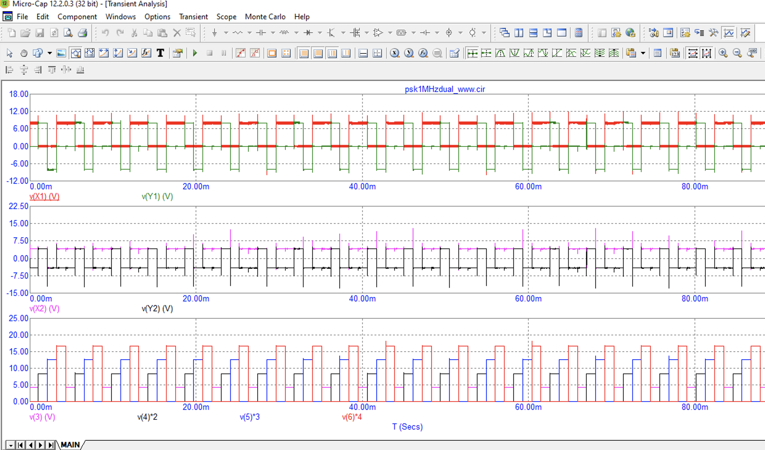
Here are some two examples: The length of the delay line (parameter TLINE::TD in the schematic) is important for the decoded symbols, because the difference phase drift between the two carriers.  

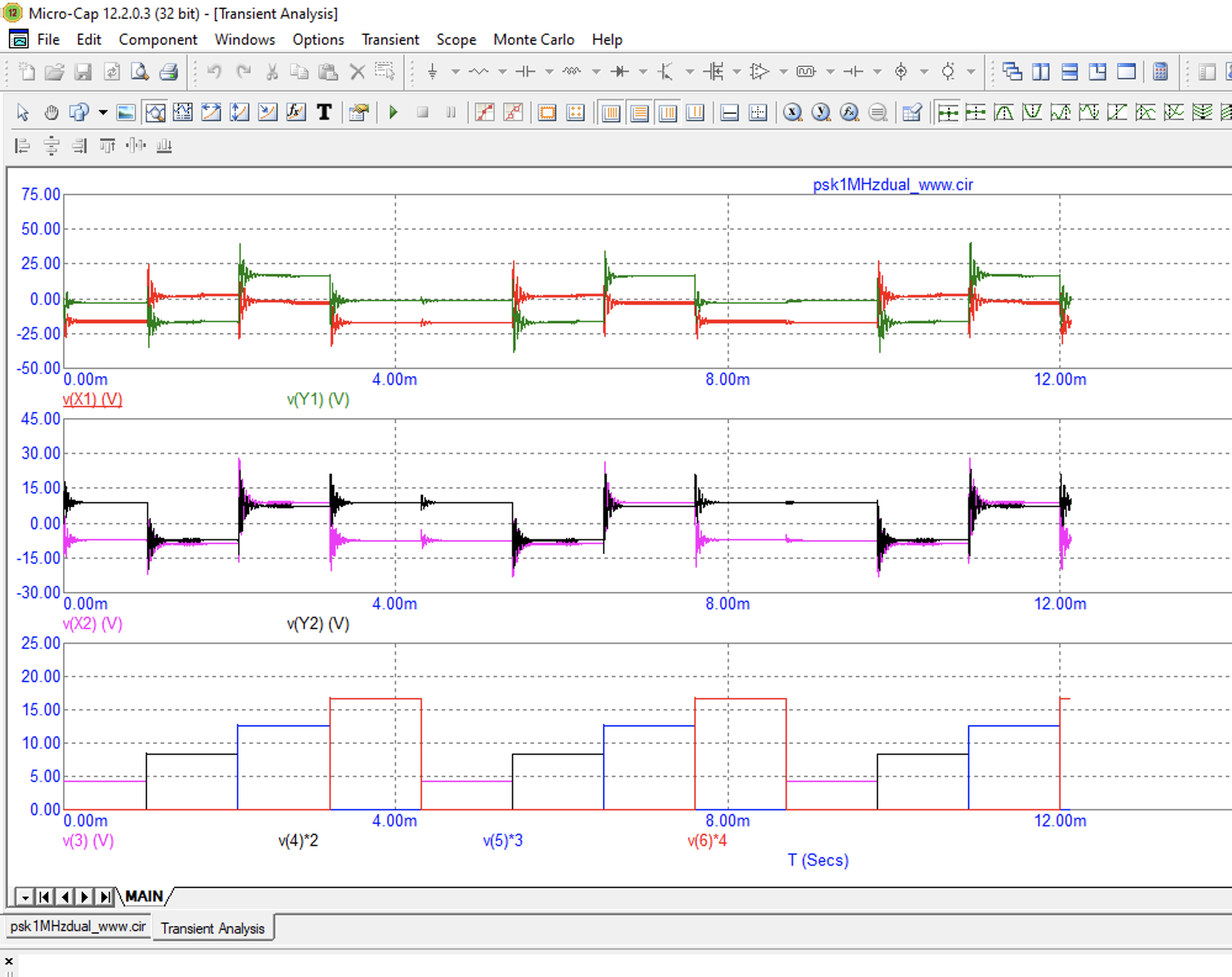
There are three graphs in each simulation, the top are the x,y decoded values for  the High frequency, in the middle  the x,y decoded values for  the Lower frequency and below the symbol that is selected: the phases are 0°, 90° , 180°, 270° but, the phaseshifts are accumulative, you really receive the symbol sequence: 0, 0+90, 0+90+180, 0+90+180+270 = 0,90,270,0 

Example 1, Carrierfrequencies 1MHz  and 500KHz.

The parameter here is FREQSPLIT  2:1.  The delay TD=0 is left (no delay) and TD=0.3333 is on the right. 

 Note that delay equal to 2/CARRIERFREQUENCY (TD=2e-6) decode the same   symbols as the case for TD=0.

 

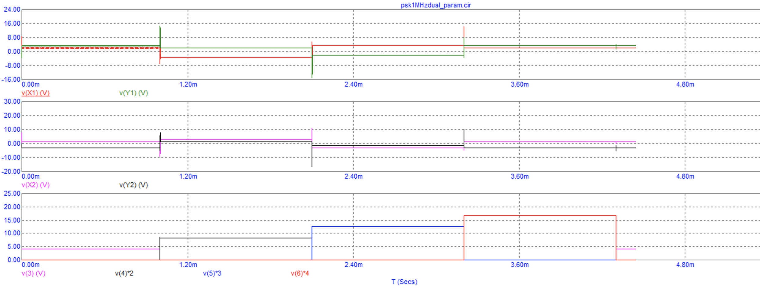
Example 2, Carrierfrequencies 1MHz  and 750KHz.

The parameter here is FREQSPLIT  4:3.  The delay TD=0 is left (no delay) and TD=1.0000e-06 is on the right. 

 Note that delay equal to TD=12/CARRIERFREQUENCY (TD=1.2000e-05) decode the same   symbols as the case for TD=0.

 

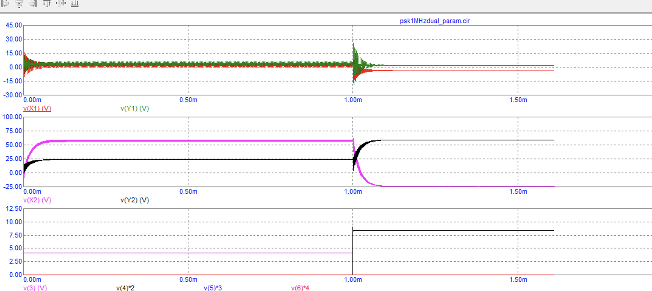
The simulation for TD=1.2000e-05 is below: the decoded values are the same as the graph on the left above!