Ionograms, the Ionospheric “Fish Finder” for HF Propagation
Holders of an Amateur Radio License are aware of the impact of the conditions in the ionosphere on the propagation of sky wave HF and VHF radio signals. Those that are regular users of the HF, have experience dealing with the regions in the ionosphere where there are varying densities of positive ions and free electrons due to solar UV and magnetic flux emissions, known as the D, E, and F layers. We may often find ourselves looking at web sites that shows the current solar emissions and HF/VHF band conditions to aid in determining which band we should be using. Or, if we should be attempting to make any distant contacts at all, by looking up the maximum usable frequency (MUF), which shows the highest radio frequency that can be expected to have ionospheric refraction.
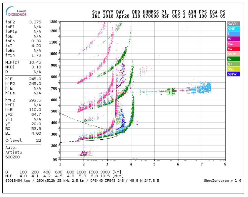
The Maximum Usable Frequency is a calculation based upon the Critical Frequency. The Critical Frequency is the magnitude of frequency that lower frequencies will have some reflection by the ionosphere back to Earth and higher frequencies will penetrate the ionosphere when they are at a vertical incidence. NOAA, Universities, USAF, International Research Laboratories, and others measure the reflections from the layers by using a ionosonde which generated radio pulses over a range of frequencies. An Ionogram is produced from traces of the recorded measured reflections. These traces of the echos form a characteristic pattern, as you can see from the ionogram shown on the first page. This ionogram, was produced on April 28th at midnight local time from the ionosonde located at Idaho National Laboratories, west of Idaho Falls. The instrument performing the measurements is a Digisonde Portable Sounder made by Lowell Digisonde International.
A historical collection of Digisonde produced ionograms from many locations can be found at the Web site, https://lgdc.uml.edu/common/DIDBFastStationList Another site produced by Serge Stroobandt, ON4AA (http://hamwaves.com/ionograms/en/index.html) has many links to and about Ionograms, includes a real-time display of the Ionogram closest to your IP address. For those of us in USA's Pacific Northwest, this will most likely be the Idaho National Labs Ionogram. The live updates will occur about once every 15 minutes. Below the Ionogram is a legend to assist in interpreting this form of Ionogram. Many of the parameters are not well explained well, so I will attempt to expand upon this legend.
Looking at the Ionogram:
X and Y Axes
The X axis represents the Frequency in Megahertz
This often comes in two different scales. At night it is often 1 to 8 MHz while during the day or when there is more ionization occurring, it is 1 to 15 MHz.
The Y axis represents the height in kilometers.
While it doesn’t make much difference for our day to day purposes, the heights are calculated heights and are discussed as being virtual heights. The term virtual height is used because RF moves slower in the presence of the atmosphere than it does in free space. So the height estimated from the time differential will be higher than the actual height.
Estimated virtual height measurements are made from the time differential between the sending of the radio pulse and the time received for each reflected frequency.
Graph Contents
The Red and Light Red traces are from the radio wave’s Ordinary Component’s reflection. The term Ordinary is used for just the reflections that are caused by the combined impact from the ionized plasma within the ionospheric layer. When high plasma levels are present in the layer the width of the trace is very thin.
The Light Red trace are single hop measurements (VO-).
Virtual height calculated from the time between the initiation of the pulse and the first measured received signal of the pulse.
The Red traces are multiple hop measurements (VO+).
Virtual height calculated from the time between the initial of the pulse and the second, third, or fourth measured received signal from the pulse.
The ionogram shown above shows up to five ordinary wave traces for the frequency between 1 and 4.25 MHz. That represents five hops where made from the initial radio pulse.
Green and Light Green traces from the radio wave’s Extraordinary Component’s reflection. The term Extraordinary is used as these are caused by the addition of the effect from Earth’s magnetic field in causing a greater refractive index impact in the ionosphere. These are not always present.
The green trace represents the height calculated from the received signals from the first hop elapsed time.
The light green trace represents the height calculated from the subsequent received signals elapsed time from the pulse.
Other Traces
Due to Doppler shift, higher frequencies are returned from the RF pulse. The color of the trace represents the direction from which the Doppler shift is coming from.
Black line traces
A trace similar to a parabolic shape intersect the Y axis twice, represents the critical frequency in respect to the true height.
A black line trace that only has one unique X value per frequency, represents the critical frequency in respect to the virtual height.
Computed Ionospheric Characteristics are presented on the left hand side of the ionogram. These are unique to the Digisonde ionograms as they are automatically computed by the software
foF2 – The critical frequency adjusted to true height for the F2 Layer in MHz.
foF1 – The critical frequency adjusted to true height for the F1 Layer in MHz.
foF1p – The predicted critical frequency for the F1 Layer in MHz.
foE – The critical frequency adjusted to true height for the E Layer in MHz.
fxI - Maximum F layer frequency in MHz.
foes - Sporadic E layer critical frequency in MHz.
fmin – Minimum F layer frequency in MHz.
MUF(D) – Maximum Usable Frequency for ground distance D. ◦ M(D) – MUF(D)/foF2
D – Ground Distance
h’F – Minimum virtual height of F trace.
h’F2 – Minimum virtual height of F2 trace.
h’E – Minimum virtual height of E trace.
hmF2 – Peak height of F2 layer.
hmF1 – Peak height of F1 layer.
hmE – Peak height of E layer.
yF2 – Half thickness of F2 layer in parabolic model.
yF1 – Half thickness of F1 layer in parabolic model.
yE – Half thickness of E layer in parabolic model.
B0 – International Reference thickness parameter.
B1 – International Reference profile shape parameter.
C-Level – Two digit confidence value
MUF versus distance chart
Maximum Usable Frequency for oblique propagation to a corresponding distance.
I looked at few historical ionograms from times of more abundant sunspots, and saw several where the traces where nearly covering the full width of the chart. I also saw a few MUF’s that were in the upper 50’s. So when these condition returns there is yet a chance I will eventually hear something on 6 meters SSB more than a few miles away.