A superb Spectrogram of an Amateur transmission on 3600kHz
Chirp Sounding Precision Carrier Analysis Ranging Techniques Digital Propagation Logging
This page is about the Ionosphere, how it was discovered, what it is, and what you can do with it. My thanks go to Dr Gary Bold ZL1AN, and the late Dr Harry Whale - the man whose name is foremost in the New Zealand history of Ionospheric Research - for help in compiling this information. In this section of the website you will also find discussions of various experiments you can do to confirm the presence and behaviour of the ionosphere. Some of these are very useful tools for monitoring and predicting propagation.
A superb Spectrogram of an Amateur transmission on 3600kHzChirp Sounding Precision Carrier Analysis Ranging Techniques Digital Propagation Logging
The Ionosphere is a fairly recent discovery. The connection between electricity and magnetism was realized by Oersted in 1819, and the theory of Electromagnetism and the prediction of radio waves was put forward by Maxwell in 1864.Hertz proved that radio waves existed in 1887, and in 1899 Marconi put radio waves to use by transmitting across the English Channel. There is some doubt as to whether Marconi really did achieve trans-Atlantic communication when he said he did, but it was soon realized that radio waves went further than line of sight, which was not at all what was expected. In 1902 Heaviside and Kennelly proposed that there must be something conductive in the upper atmosphere that caused signals to be returned to earth at great distances.
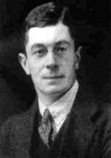
Things moved on apace from there. Edward Appleton (pictured here) proved that the ionosphere existed by measuring wave fronts, and also in 1926 Breit & Tuve made the first radar-like machine to probe the ionosphere - the first ionosonde. In 1926 radar man Watson-Watt first proposed the name "ionosphere" for the Kennelly - Heaviside layer, and in 1927 Sydney Chapman (pictured above) proposed his now famous mathematical model of the ionosphere. 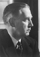
Edward Appleton (left) and Sydney Chapman (right)The first satellite, Sputnik 1, caused an absolute sensation in 1957, when its signals on 20 and 40MHz could be heard when the satellite was on the other side of the earth! The Canadian Alouette satellites were the first to provide ionospheric sounding from above the ionosphere.
Very important Ionospheric Research work was carried out in New Zealand. Because of its isolation from Europe, made all the more apparent by WWII, the Defence Dept and the Post Office persuaded the government to invest in research, in order to find out how better to maintain military, commercial and broadcasting links to Europe. Previous research had been related to propagation over shorter distances, and nothing was known about antipodal propagation, auroral zones and long path, all of which are important factors to long distance communication.
The Seagrove Radio Research Station was set up by the DSIR and Auckland University in 1950. The first director at Seagrove was Dr Harry Whale, at the time undertaking post-graduate studies in Cambridge (at the famous Cavendish Lab) on the same scholarship awarded to Ernest Rutherford.
The first Rotating Interferometer at Seagrove (sketch by Dr Harry Whale)
(Click on image for larger view)Around 1951 Dr Whale started to develop the world's first instrument capable of resolving the arrival direction and elevation angle of radio waves. It took some two years to develop, and the sketch shown here, from Dr Whale's own book, shows that first machine. It consisted of a fixed antenna on a tower, and a rotating antenna which travelled on a trolley around it, on a circular track of about 120m diameter. The antennae were top-loaded verticals about 6m high.
The interferometer used two receivers inside the shack, connected to a specially built amplifier and phase detector, which caused marks to be scribed on a blackened drum which rotated with the antenna array. In addition to propagation research, this deceptively simple equipment was used to track early Russian and American satellites. All measurements involved vast amounts of data analysis with log book, adding machine and slide rule.
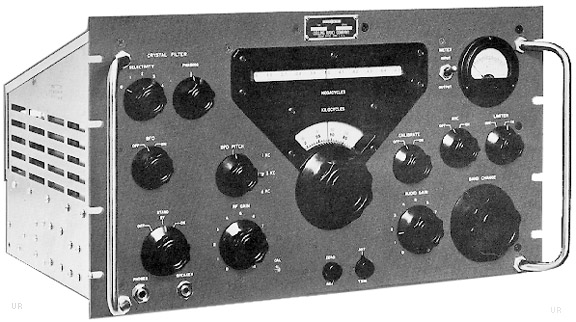
The superb Collins 51-J4 HF ReceiverThe first receivers used with the Interferometer were National HRO models, later replaced by the much superior Collins 51-J4 (illustrated above). ZL1BPU has one of these fine receivers used first at Seagrove and later at Ardmore in his shack, unmodified and still working perfectly after 55 years.
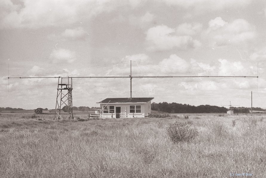
The Ardmore Interferometers (photo by Dr Gary Bold)In the 1960s two new Rotating Interferometers were constructed at Ardmore, smaller than the one at Seagrove, but of much better construction, with both antennae rotating. The large one in the foreground of this photograph, was 40m in diameter, with 4m vertical dipole antennas at each end. In the background at the right can be seen an even smaller interferometer, which rotated more quickly and was used to track satellites. An adaptation of this type of equipment is still used today for direction-finding on VHF.
In the late 1960s Dr John Titheridge was working at Ardmore. Dr Whale was for a time seconded to NASA, where he advised the space program on propagation matters.
Starting in 1957, for the International Geophysical Year, many pulse ionosondes were installed around the world, including the one pictured at Ardmore (photo by Dr Gary Bold). The antenna typically consisted of two broad-band loaded inverted vees, at right-angles, one for the transmitter, the other for the receiver. The transmitter in the hut had about 600W peak output and mechanically tracked with the receiver and recording camera from 1.5 to 16MHz.
Many clever techniques which give information about the ionosphere have been developed in the years since IGY. Specialized ionospheric sounding equipment is now routinely used by military, commercial and research agencies for propagation studies. Some simple techniques for studying the ionosphere, which are easily reproduced by Amateurs, are described on this site.
The formation of the Ionosphere depends firstly, and most importantly, on the sun. The earth is bombarded continually by high energy radiation, travelling of course at the speed of light, and by high speed solar particles, mostly charged, which also travel at fairly high speed. Because the earth is moving through this soup of high speed particles, a supersonic shock wave is formed. The charged high speed particles, called the 'solar wind', would pass through the ionosphere and cause us much damage if it was not for the earth's magnetic field, which is in turn present only because the earth (uniquely) has a molten iron core. Because the solar wind particles are charged, they are deflected around the earth by the magnetic field. Some enter the polar regions to form the auroral layers, but the Magnetosphere, the area where the earth's magnetic field is active, deflects most particles away. The Magnetosphere is very large, stretching well beyond the moon.You might think that the ionization of the upper atmosphere is caused solely by the trapped solar particles, but this is only a minor effect. Most of the upper atmosphere ionization results from the interaction with the upper atmosphere gases by powerful UV and X-Rays, which are not affected by the magnetic field. Electrons are split from these gas atoms, leaving active and highly mobile electrons and larger less mobile charged ions. The area of ionization extends from about 60km above the earth, out to about 500km.
It must be fairly obvious that as the pressure in the atmosphere decreases with altitude, so also does the density of the air, reducing the number of atoms per unit volume. This effect is shown in the first graph (right), which illustrates typical gas density against height in km.
The sun bombards us from above with electromagnetic rays that are absorbed when they hit atoms, and so, as illustrated in the second graph (radiation intensity versus height in km), the radiation intensity is highest at high altitude, and decreases to almost nothing at the surface of the earth.
We now know a little about the mechanism for refraction from the ionosphere. When a radio wave reaches the ionosphere, the electric field in the wave forces the electrons in the ionosphere into oscillation at the same frequency as the radio wave. Some of the RF energy is given up to this resonant oscillation. The oscillating electrons may either recombine, losing the radio energy, or will re-radiate the original wave energy. Total refraction can occur when the ion collision rate (recombination) is less than the radio frequency, and if the electron density in the ionosphere is great enough.
That said, the mechanism is significantly complicated by differing ion density at different heights, and different chemistry involved in each refracting layer.
Imagine, as Sydney Chapman did, that there must be some relationship that expresses the combination of these two effects. There must be some point, illustrated in the third graph, where the balance of high enough numbers of atoms is balanced with still high enough radiation, and a peak should be expected in the level of ionization of the atmosphere. You see this in the third graph, peaking at about 300km.New ions are formed by bombardment, and older ones decay as they meet up with free electrons. This fine balance affects the amount of ionization present at any time.
In this combined graph, the three curves have been superimposed to show how the broad band of ionization comes about. Of course reality is a lot more complex than the simplest models. The electron density is never uniform, or has just one peak, as indicated here, and because it tends to have several different peaks in density, a wide range of effects can occur.
As indicated in this graph, the refractive index, or the ratio of speed of light in the medium compared with that of space, also depends directly on the electron density.
Because the energy from the sun varies daily and seasonally, the ionosphere is never static. The sun also has times of extreme activity, causing storms and severe disruption to propagation.
The ionosphere is far from homogeneous, and not only does the amount of charge vary with height, but so does the mixture of gases, as illustrated in the picture. Because at different heights different gases are present, and because at these heights different solar radiation may be available, different chemical reactions take place.
As previously mentioned, the rate of ionization depends on the density of atoms and intensity of radiation, but it also depends on the actual chemistry involved. Some reactions take place quickly, or cause higher ionization, while others act more slowly or result in less ionization.
The rate of subsequent recombination depends only on the density of the ionosphere (how close the atoms are), and what the chemical process is. The sun has little to do with it. So, the electron concentration varies with height, giving us different layers, affected in different ways by the sun, and with different radio properties.
Refraction occurs because ionized molecules have free electrons which are able to vibrate in response to the arriving radio signal's electric field, like tiny dipole antennas.
Radio waves are bent away from areas of high ionization because these areas have a lower refractive index. The bending effect is reduced as the frequency of the radio waves increases, and then suddenly stops, so the waves pass on through (above the critical frequency).
The speed of the radio waves also depends on the refractive index (ion density), and also on the angle of arrival at the reflective layer. Steeply angled waves are more likely to pass through than those at a grazing angle.
Because spinning electrons are affected by the earth's magnetic field, they tend not to spin in circles, but in ellipses. The effect is most marked at the poles, where the magnetic field is more concentrated. This has the unusual effect that the refeactive index differs for different wave angles.
As a result, it is quite normal for a radio wave to have its polarization changed by the ionosphere, and furthermore, for waves of different polarization to be refracted different amounts. This leads to the return to earth of two different rays (the Ordinary and Extraordinary rays) with distinct properties. Just as with reflections from other layers or at other times, these rays can have slightly different frequencies, phase, amplitude and time of arrival.
On the right you see an example of F-layer propagation on 3.5MHz. In this spectrogram, which displays frequency vertically and time horizontally, you can clearly see that the signal frequency varies all the time, and that towards the right there are clearly two related but distinct F-layer rays recorded. (The two rays recorded at the left, over the sunset period, do not have related behaviour. They are E-layer and F layer and can be seen to behave differently).
So, as you see, in reality the situation is very complex, and never static. The ionized layers have different densities, different levels of ionization, and so have different refractive properties (bend radio waves differently), even in different directions and planes. When conditions are suitable, radio waves can be bent so that they travel along inside the ionosphere, or are bent right back to return to earth. At other times, other frequencies, or with other layers, the waves can be passed straight through or be absorbed by the ionosphere.
The best known layers have conventionally been named with letters of the alphabet.
F Layers
The F layers are the most widely used for HF propagation, but are also the most complex and most strongly affected by solar behaviour. There tends to be just one strong F layer at night, at around 300 - 500km altitude. This layer is generally stable and slowly fades as the night progresses. This layer is caused by UV bombardment, which ionizes atomic Oxygen.During the day, the F layer becomes much more highly ionized, is much more active, and spreads down to a lower level (about 200 - 300km) where a second layer with slightly different chemistry exists in addition to a highly volatile upper layer, at around 300 - 500km.
F layer refraction depends on the level of ionisation, and higher frequencies require higher levels of ionisation. The F layer is generally active from about 3 MHz to 10 MHz, but can extend beyond 30 MHz. During the day, lower frequency access to the F layer is impeded by the (lower altitude) absorbing D layer. Whether a radio wave is refracted or passes striaght through these layers, depends on the angle of the wave arrival.
E Layer
This layer is at about 100 - 120km altitude, is generally stable, and weakens or disappears at night. The layer is generated by soft X-rays and far UV, which ionise molecular Oxygen, O2. Unusual and unpredictable patches of strong ionization are not uncommon in the E layer.D Layer
This is the lowest of the layers which affect HF propagation (75 - 90km). It is a strong attenuator of signals up to about 8MHz, preventing these signals from reaching the higher layers. The D layer has no reflective properties. The D layer is active during the daytime, is slow to form (up to two hours after sunrise), and quickly dissipates at sunset. This layer is responsible for preventing long distance communication during the day up to about 8 MHz.The chemistry of the D layer involves ionisation of Nitric Oxide (NO) by UV Hydrogen emission, and by hard X-rays. Recombination rates of ions in the D layer are high, because the atomic density is high, resulting in more neutral air molecules than ions. MF and low HF radio waves are markedly reduced in strength by the D layer, as the induced electron motion causes energy loss through frequent collisions.
The D layer loses charge quickly after sunset, then allowing signals to reach the higher refractive layers. At times of unusual solar events (solar proton storms), the D layer reaches very high levels of ionisation, which can cause widespread radio 'blackouts'. These especially affect trans-polar radio paths, as this extreme ionisation is funneled to these regions by the Earth's magnetic field. These 'blackouts' can last one or two days.
Multi-path Propagation
Reflections can take place between these layers, as well as reflecting from the earth and grazing ('chordal hop') reflections within one layer, making the situation very complex. Chordal hop is believed to be a major reason for the strong signals experienced over night-time paths, as there is less attenuation than is involved in reflections from the earth. Signals over long distances are thus frequently stronger and more stable going around the world through the longer night-time path ('long path') than the shorter daytime path ('short path').
Skip
Ground wave propagation of radio signals is of course limited by the curvature of the earth. While lower frequency radio waves (say below 500kHz) can follow the terrain and have long useful ground wave ranges, higher frequencies cannot be heard via a direct signal very far at all. Ground wave is typically about 50km at 3.5MHz and can be as little as 5km on 20MHz. A useful rule-of-thumb is that the ground wave range is typically about 500 wavelengths.Vertical waves penetrate the ionosphere further than oblique waves, and are also slowed (delayed) more than oblique waves. Waves arriving near vertically escape through the ionosphere first, leaving no reflected signal, so the critical frequency (frequency above which the signal escapes) is lower at higher incident angles.
At the lowest frequencies, even vertical waves are reflected ('Near Vertical Incidence Signals' or NVIS), unless the ionization becomes very weak (say late at night), or the signals are absorbed by a lower layer.
You can see therefore that longer distance HF communication relies heavily on ionospheric refraction, and that the frequency and time of day must be chosen carefully so that propagation occurs to the target location.
However, there is a snag - as described above, to reflect a signal to further away is a reasonable proposition, but at shorter distances, the radio wave has to travel at a steep angle into the ionosphere in order to return to the target receiver. Since the steeper waves tend not to be reflected, it is not at all uncommon for there to be a zone around the transmitting location where the signal is not heard at all!
This area (called the 'skip zone') is the area outside ground wave range where the sky wave is not reflected by any ionospheric mechanism. The radius of this area (at HF) can be between 500 and 2500km. In the area between ground wave range and the skip distance where the the first ionospheric reflection arrives, the signal may not be heard at all!
In practice the signal may be detected in this area via a scattering mechanism, but these signals tend to be weak, unfocussed and highly unpredictable. (Unfocussed signals are those arriving from a multitude of short-term points of reflection, and have very poor phase coherence. They can be likened to the reflection of sunlight off ripples on a pond, and are directly analagous to scintillation - flickering - of light from distant stars).
Sometimes signals are received in the skip zone by reflection off other objects (aircraft, meteorites). The skip zone can be put to good use in studying these effects since the ground wave and ionospheric path signals are much weaker that these reflections, which also exibit considerable Doppler frequency shift.
Multipath Reception
At any one time, signals can be arriving at the receiver via a multitude of different paths. Each of these paths has different properties, and so the arriving signals will have different phase (and so add or subtract at the receiver), different signal strengths, different polarizations and - most significantly - different times of arrival. The different paths may have delays as great as 60ms or more. On the higher HF frequencies the longest delay differences are caused by a mixture of long path and short path rays (the effects can be minimized by using directional antennae). On lower HF frequencies, NVIS propagation causes the sky wave to be seriously delayed compared with the ground wave.Signals may be very strong when there are many rays arriving at the receiver, but after just a few seconds the signal phases may change, causing a deep fade. These affects are dependent on frequency, and so it is found that these deep fades are highly frequency selective (called 'selective fading').
Strong fading is experienced near sunrise and sunset, when on high frequencies E and F-layer signals arrive together, and on lower frequencies when E-layer and ground wave arrive together. Because the fades can be frequency selective, it is common for parts of a radio signal to be attenuated, while other parts are not. This is the cause of severe distortion on AM broadcast signals, where the carrier is attenuated and the receiver has not enough carrier to demodulate the sidebands, leading to apparent over-modulation and second harmonic distortion. SSB signals and narrow-band signals such as Morse are subjectively less affected.
Wide digital signals also suffer from this effect, and need to be designed to compensate for selective fading. The picture to the right shows selective fades passing through a 1kHz wide digital signal on 14MHz. At a range of 2500km, the mechanism is probably the interaction of F1 and F2 layer signals. Other digital modes are designed to be narrow enough that selective fading hopefully affects all the signal at the same time, and have sufficient sensitivity and error correction to ride through the fades.
Another effect caused by multipath signals is related to the difference in time of arrival. Although from time to time voice signals with echo and Morse signals with a "mushy" or indistinct sound are heard, by far the biggest problem caused by differential timing is the effect on digital modes. For example, imagine an RTTY transmission using 50 baud (20ms signalling elements) in a situation where there is 10ms difference between two paths that vary in strength. The received signal will be erratically delayed or advanced by 10ms, causing individual signalling elements to be made indistinct by superimposition of an earlier or later element. Many techniques have been developed to overcome this problem, but generally the best approach is to slow the signalling elements so that the timing differences are small compared with the element length. MFSK is an especially suitable technique for such conditions (MFSK16 or FSQ for example).
Chordal Hop
When a signal approaches the ionosphere at a steep angle the signal penetrates the ionosphere and may pass right through, or be 'reflected' back (green ray, right). It is actually refracted rather than reflected. However, when a signal approaches the ionosphere at a grazing angle, the likelihood of 'reflection' is higher than for vertically approaching signals. The penetration is less and the attenuation is less. Further, if the angle is low enough, the signal can be reflected again off the ionosphere without first hitting the ground (red ray, right).
This 'chordal hop' process is believed to be common at night when the F layer is stable. Because there is no ground reflection involved, and less penetration of the ionosphere, the attenuation is much less than with other propagation mechanisms, and as a result signals are stronger. In order to enhance the possibility of Chordal Hop, it is important to make use of antennas with the lowest possible beam elevation, to ensure that the signal hits the ionosphere as far from the transmitter as possible.
Grey Line
One much discussed, but poorly documented, process affects propagation of low LF and MF signals at a time of day when the transmitting station and receiving station are in the dawn or dusk twilight period. The mechanism is not well understood, but plenty of anecdotal evidence is available to show that good DX can be worked on 80m and 160m in particular at this time of day. An interesting paper by Steve Nichols G0KYA discusses some experiments designed to measure the effect.The Twilight Zone revisited - recent grey-line research Steve Nichols G0KYA July 2005
Some of the properties of the ionosphere can be predicted in general terms over relatively long periods. As is widely known, the sun's activity varies over an 11-year cycle, with some evidence of an additional 22-year cycle. Since the ionization of the upper atmosphere depends on particles and radiation from the sun, this ionization also follows periods of more or less activity. When activity is high, there is a higher likelihood of magnetic storms, which can cause blackouts (the ionosphere stops 'reflecting') and times of very high ionization and hence very good propagation at very high frequencies, right up into low VHF. At these times the D layer is also highly ionized and low frequency propagation during the day is especially poor.When solar activity is low, ionization is low and the ionosphere generally more stable. Higher frequency operation is less likely except when daily activity is optimum, but lower frequency daytime propagation is improved.
As previously described, there are also daily variations as the earth rotates, and there are also season changes as the earth's tilt angle to the sun changes. Solar performance has been monitored for several hundred years, through the simple experdiet of counting sunspots. The sun is now continually monitored via numerous terrestrial and space-based measurements of particles, and in visible, infra-red, ultra-violet and radio spectra. From these measurements various solar and ionospheric predictions are made based on complex mathematical models.
Even with modern sophisticated monitoring, the sun still comes up with surprises, such as flares, magnetic storms and unexpected sunspots. Some apparently predictable effects such as the diurnal change in MUF also cause sudden loss or enhancement of propagation, and clouds of uneven ionization in the E layer can cause unexpected propagation. In addition, other effects that do not depend on the sun directly can affect propagation in an unpredictable way. Many of these make fascinating subjects for study, as simple equipment is all that is necessary.Sporadic E
This enhanced propagation is caused by high levels of ionization in relatively localized areas. The cause is unknown, and the results can be spectacular, leading to good DX on higher bands, even into VHF. The ionized area may be only 100km or so across, so the effect is like having your own mirror - as the day progresses, the mirror moves and gives you access to different destinations. These layers come and go without warning and can last minutes to days. It is difficult to monitor for Sporadic E, but it is well worth while making use of it! MEPT-JT database analysis can show when these events may have occurred, and suggest target stations to monitor for future events.Sudden Disturbances
Usually caused by solar storms, these disturbances occur because the ionosphere becomes bombarded by high energy particles from the sun, upsetting the balance of chemistry and ionization for periods from minutes to days. Sometimes propagation is enhanced, but very frequently propagation on the higher bands is impaired or lost completely, while lower bands signals develop a strange raspy quality and there is more noise. Sometimes propagation is enhanced briefly as well. These disturbances can now be predicted reasonably well, as the solar flare that causes them can be seen in the UV spectrum well before the ionized particles arrive.These disturbances can be monitored by routinely measuring the strength of HF broadcast stations over a wide range of frequencies. Build up a pattern of average strength at various times of day over several weeks. A sudden and unexpected change in strength is a sure indication of a disturbance. Preferably use stations which operate 24 hours on the same frequency (for example WWV).
MUF Dips
If you follow propagation predictions you can get a reasonable idea of when propagation on a particular frequency in a particular direction will fail. However, if you choose to operate very close to the MUF, daily variations will sometimes lead to surprises, especially under NVIS conditions when the signals are more likely to escape through the ionosphere. For example, over a 10km path on 80m at night, it is normal for F-layer propagation to exist all night, but sometimes (picture below) there are surprises, when slightly poorer ionization and lower MUF causes propagation to be lost in a spectacular way.In this picture, F layer propagation is lost between 0430 and 0630 (early morning), leaving ground wave as the only propagation path. As propagation peters out when the MUF becomes too low, the polarization effects become very marked, and the two O and E rays fade out separately 40 minutes apart, and with different Doppler shift. When the F-layer signal returns there is much scatter, the frequency is higher (because the reflective layer is lowering as the sun hits it), and there are clearly three propagation paths, caused by zero, one and two reflections off the earth, and one, two and three refractions from the same area of the ionosphere.
Some ionospheric effects are very obvious on all transmissions (selective fading, back scatter, and so on), but some effects are quite small, and like those illustrated in the picture above, can only be detected using very stable signals with minimal modulation, or at least very stable carriers and no modulation close to the carrier (hence a well designed AM broadcast transmitter is appropriate, although few are stable enough). The transmissions should not have phase or frequency modulation, phase noise, keying or unwanted sidebands which would obscure the observations. Traditionally, the standard frequency transmissions of CHU, WWV, WWVH, VNG and the like have been used for this purpose, and Amateur super-stable transmitters have also been designed (such as the ZL1BPU GPS locked transmitter used to obtain the previous picture).There are two main effects that can be observed using such stable transmissions. These are Doppler effects and Polarization effects. On occasions dramatic frequency shifts due to solar flares are also to be observed. As with all HF transmissions, you will also frequently see Scatter (scintillation) under the signals. Meteor Scatter can also be observed, but the effect is small on 80m. The picture that follows (recorded on 17.675MHz) shows some meteor reflections - as little dots and srokes above and below the carrier of Radio New Zealand International (in skip), and has a spectacular solar flare effect showing at the right. Just to the right of the flare is a hook-shaped Meteor Scatter reflection.
Meteor scatter and a flare (to the right)
(Click on image to enlarge)Of these effects, Doppler has the most effect on the accuracy of of-air frequency measurements. Signals that are in skip and show scatter are most strongly affected by Doppler.
Doppler
The Doppler effect is well known. However, not many Amateurs realize that changes in the ionosphere can cause measureable changes in observed frequency and phase of radio transmissions. The ionosphere's ion density varies all the time, due mostly to time of day (angle of the ionosphere to the sun), temperature (affects ion density) and solar activity, which causes the charged particles in the first place. As a result, the altitude at which any frequency is refracted back by the ionosphere changes as the ion density and therefore refractive index changes. In general the effect is small (less than 1 part in 106 or 1Hz per MHz), but is greater with scattered signals and can be spectacular during solar flares and around sunrise and sunset.
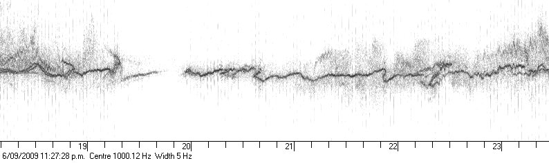
An example of Doppler Effect on Carrier Frequency
(Click on image to enlarge)In this picture, spanning some three hours (horizontal scale) the transmission from ZL1MT on exactly 3600kHz appears to have moved up and down about 2Hz (the vertical scale is 5Hz top to bottom). At times the frequency changes quite quickly. Note that the transmitter and receiver frequencies have not changed - it is the apparent received frequency that changes. Sometimes the apparent frequency is above or below the true frequency for hours on end!
When making frequency measurements on signals experiencing Doppler, take readings over an extended period of time, at different times of the day, and over several days, in order to determine what you consider to be the mean frequency. If within ground wave range, make the measurements when sky wave is less likely to affect the signal. Even though often very weak, daytime E-layer propagation is more reliable for frequency measurement, as it experiences much less Doppler.
Polarization
The refractive index of the ionosphere differs at different heights, so for rays arriving at different angles to the refractive layer, different penetration and delays are caused at different angles, hence the NVIS - Near Vertical Incidence Signal - delay and fading effects.
The effect is most marked when the signal is close to the MUF (Maximum Usable Frequency), is crossing a polar region, or when the ionosphere is changing quickly. What happens is that the various components of the signal appear to arrive on different frequencies!
In the picture above you can see this effect at around 2230. The signal has apparently split into several paths. Usually one ray will predominate - this is the "ordinary ray", and is the only ray visible most of the time. On occasions one or more fainter "extraordinary rays" will appear, either higher or lower in frequency. These rays frequently appear to intermodulate, (this can be caused in the receiver, especially if AGC is active) so you will see in the above example the extraordinary rays are equally spaced about the ordinary ray.
In the next small example, the Ordinary and Extraordinary Rays are really spectacular! This is a transmission from ZL1BPU, received by ZL2AFP at 400km range and was recorded mid-evening on 80m using the same settings as the previous picture.
Spectactular O and E Rays (and many other effects) on 80m, 400km rangeTransmitter power was 1W, and the transmitter GPS locked. Vertical stripes were caused by FSK Morse ID. Here you see O & E around 1830 hrs, with one ray folding back at 1850 hrs, F-layer drop-out at 1950 - 2000 hrs, and a most complicated O&E foldback at around 2220 hrs!
Scatter
Scatter occurs when signals are reflected from rough details on the earth's surface, or from 'ripples' in the ionosphere. When the signal appears back in the direction it has come, it is called 'back scatter'. Since the reflections are from irregular and unstable objects, when they arrive at the receiver they can be on different frequencies, and tend to form a cloud around the signal. If the main signal is not propagated to the receiver, all you may get is scatter. This is normally what we receive in the South Pacific from WWVH, which explains why it is no real use for frequency measurement and comparison, although the audio may sound fine, even though the signal is weak. In the previous image you can see scatter mostly above the signal as a fuzzy cloud. It is normal for the scatter to be markedly more frequency shifted than the main signal, and always in the same direction.Observed on a spectrum analyser, the scattered signals appear to be stable, strong, and focussed, and yet they move around a lot. As a result, the slower integration time of a spectrogram tends to show noise rather than a focussed signal. The mechanism of scatter is very similar to scintillation of star when observed through the atmosphere.
The next image shows scatter on the carrier of ZLXA (Levin) on 3935kHz. This transmitter is not stable enough for precision measurement, but exhibits good scatter, and is on 24 hours a day, and of course near 80m.
In monitoring ZLXA you will see different effects every day. Often the sky wave arriving after sunrise is preceded by backscatter from somewhere East of the path where the sun is already up - giving a ghostly foretaste of what is to come perhaps 10 minutes before the sky wave carrier arrives. As the D layer is energized at sunrise, it often enhances sky wave for a period before it absorbs completely, perhaps due to upward reflection from the top of the D layer.
Backscatter on ZLXA
(Click on image to enlarge)This signal was recorded at around sunrise. Note how the backscatter "clouds" are sometimes above the carrier frequency, and sometimes below, since the path to the receiver from the backscatter source is quite different to the forward signal. Some O and E Rays are also visible on the scattered signal. The width of this picture is 10Hz, so the effect is about �2ppm wide.
Provided scatter is not accompanied by excessive Doppler, measurements of modest accuracy can be made by measuring the centre of the fuzzy signal. Unfortunately this is not usually the case (see the above example), and measurements on DX signals such as WWV and WWVH are fraught with problems.