 Antenna System
Measurements with the MFJ-202B RX Noise BridgeAntenna System
Measurements with the MFJ-202B RX Noise Bridge
Antenna System
Measurements with the MFJ-202B RX Noise BridgeAntenna System
Measurements with the MFJ-202B RX Noise Bridge
INTRODUCTIONIn the 1970's and 80's, antenna noise bridges, also known as RX noise bridges such as the Heathkit HD-1422, Palomar Engineers R-X and the MFJ-202 became commercially available to the amateur radio community. These devices are used with an external receiver to measure unknown impedances and consist of a broadband noise generator and a bridge circuit with a calibrated variable capacitor and resistor. These noise bridges can directly determine the resonant (zero reactance) frequency of an antenna or other unknown, but determining other impedance values often requires complex calculations. As microprocessor technology has made possible digital antenna analyzers and vector network analyzers that perform these calculations, RX noise bridges are now commonly found for sale at reduced prices. These notes describe the use of spreadsheet utility for calibration and measurements of an antenna and a zip cord transmission line with an RX noise bridge. |
|
In operation, a receiver is connected through a 50 ohm coaxial cable to the "RECEIVER" connector on the noise bridge, tuned to the desired frequency and set to the AM mode.. If the radio is a transceiver, the transmitter should be disabled by reducing the power level to zero to prevent accidental transmission that could damage the noise bridge. The unknown impedance is connected to the "UNKNOWN" connector and the resistance and reactance controls are adjusted for a null (minimum noise) in the receiver. The receiver's automatic gain control (AGC) should be set to the "slow" or "off" position because the AGC action may render the null difficult to detect. If a null still cannot be detected, one may also need to activate the attenuator and decrease the RF gain of the receiver.
| Range expander off | Range expander on | ||||
|---|---|---|---|---|---|
|
|
|
|
1 MHz | 4 MHz |
|
|
|
|
|
|
|
|
|
|
|
|
|
|
|
|
|
|
|
|||
The manual states that the MFJ-202B is not a precision grade laboratory instrument, but its accuracy may be improved by calibrating the dials. The schematic diagram shows the controls are a 250 ohm variable resistor and a 10-300 pF variable capacitor. The resistance dial is marked from A through G, and the reactance dial is marked in pF from 150 XL, through zero, to 150 XC. The range expander switch inserts a 200 ohm resistor in parallel with the unknown impedance to be measured.
To zero the reactance dial, the receiver was set to 2 MHz and a short piece of wire was connected directly between the center conductor and the ground threads on the "UNKNOWN" connector. With the range expander switch in the "Normal" position, both resistance and reactance controls were adjusted for a null in the receiver noise. The resistance control was near "A" or "zero" ohms. If the reactance knob did not read "zero", the knob set screw was loosened and reset to the "zero" mark. Grebenkemper2 described a case in which the "zero" reactance setting varied with frequency due to bridge imbalance and a method to remedy this and to accurately calibrate the reactance scale.
To calibrate the resistance dial, a few non-inductive (carbon
composition or metal film) resistors of known value
throughout the range from 0 to 250 ohms were used.
Alternatively, a small potentiometer may be used. A digital
multimeter was used to accurately measure the values of the
resistors. The resistance knob set screw was loosened and
reset to the "A" mark at the limit of counterclockwise
rotation. With the expander switch in the "Normal" position
and the reactance control at "zero", each resistor was connected
using the shortest possible lead length between the center
conductor and the ground threads on the "UNKNOWN" connector and
the corresponding resistance knob position was recorded for each
null in the receiver noise. The resistance dial readings
were converted from the alphabetical "A" through "G" to a
corresponding numeric scale "0" through "6". These
measurements listed in Table 2 and plotted graphically in Figure
1.
|
 |
||||||||||||||||||
|
readings for known resistances |
dial readings for known resistances |
||||||||||||||||||
|---|---|---|---|---|---|---|---|---|---|---|---|---|---|---|---|---|---|---|---|
This data was entered into a spreadsheet (Figure 2) to perform a linear regression analysis.3 Download Microsoft Excel spreadsheet. This determined the relationship between the unknown resistance and dial scale to be:
|
|
TRANSMISSION LINE MEASUREMENTSIn his article, Grebenkemper2 described various R-X noise bridge applications in various measurements of antenna and transmission line characteristics. Banz4, Duffy5, Jurgens6, Maguire7, Schmidt8, and Straw9 have published computer programs and De Stefano10 has published a series of video tutorials for these applications. Figure 4 shows the spreadsheet used to calculate the characteristics of a 36 foot (11 m) length of Pfanstiehl 18-gauge AS-18/50Z PVC speaker wire used as transmission line.11 Hall12, Parmley13, and Wiesen14 have previously discussed and characterized the use of other zip cords as transmission lines.To determine its velocity factor (VF), a 78.25 inch (1.987 m) random length of the speaker wire was attached to the UNKNOWN connector of the noise bridge. The frequency at which the line was a quarter wavelength long (zero reactance) was then determined for when the conductors far end were open and when they were shorted together, and the mean of the two frequencies was calculated (24.99 MHz). The velocity factor (VF) at that frequency was then calculated as the ratio of the length of the line to a free space quarter wavelength, or 0.66. The dielectric constant (k) is the reciprocal of the square of the velocity factor, or 2.3. VF = 4 × λ/4 length(m) × fMHz/299.79 and k = 1/(VF2) |
 |
| Fig. 3.
Pfanstiehl 18-gauge AS-18/50Z Speaker Wire |
|---|
The characteristic impedance (Z0) of this random length of speaker wire transmission line was then determined by measuring its impedances with the far ends open and shorted, and taking the square root of the product of those numbers. It was found that these impedances fell within the range of the noise bridge at 5 MHz and 7 MHz. The characteristic impedance was calculated as 114.4 ohms at both these frequencies. In the particular case of a parallel transmission line, this result was confirmed using the formula for calculating Z0 from the physical dimensions of the parallel transmission line. Substituting 114.4 ohms for Z0 and the 0.512 mm radius (r) of the 18 AWG conductors, gave a center to center conductor separation distance (D) of 2.2 mm which was confirmed by physical measurement of the wire.
Z0 = √(Zoc × Zsc) and Z0 = 276/√k × log(D/r), D = 10((Z0×√k)/276+log(r))
The electrical length of the full 36 foot speaker wire transmission line used with the 40 meter horizontal loop antenna15 was determined by disconnecting it from the antenna and shorting those ends together and attaching the noise bridge to the station end of the feed line. The feed line was determined to be 0.5, 1 and 1.5 wavelength long at 9, 18.25 and 27.7 MHz, the first 3 frequencies at which the reactance was zero and the resistance near zero. These frequencies were observed not to be exact multiples, reflecting the velocity factor variation with frequency. Using the previously calculated velocity factor of 0.66 at 24.99 MHz, the physical length line of this feed line (one electrical wavelength long at 27.7 MHz) corresponded to 35.3 feet (10.8 m). The feed line loss at 27.7 MHz αl(f0) was calculated as 8.69 times the ratio of the measured resistance Ri to R0, the resistive part of the characteristic impedance Z0. The feed line loss at other frequencies αl(f) was estimated by multiplying αl(f0) by the square root of the ratio of the frequencies.
λ length(m) = VF × 299.79 /fMHz
αl = 8.69 × Ri/R0 and αl(f) = αl(f0) × √(f/f0)
|
|
|
|
|
|
 |
 |
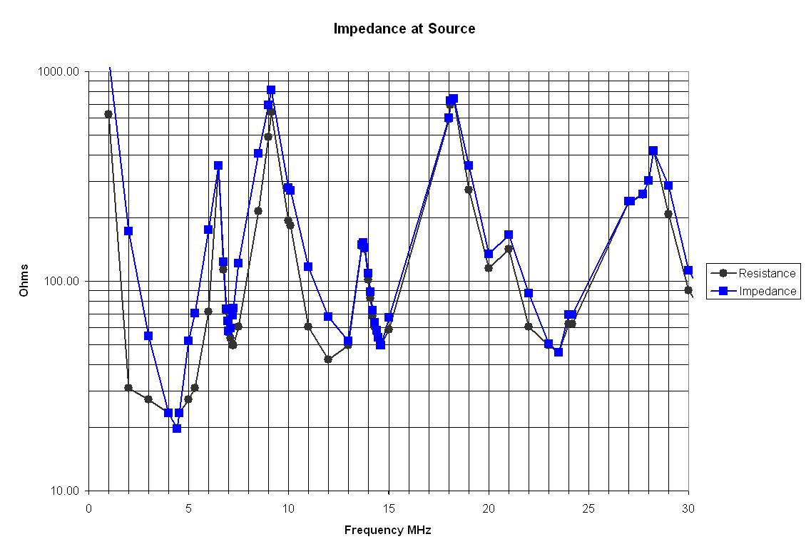
| Figure
7. Measured Impedance at Source |
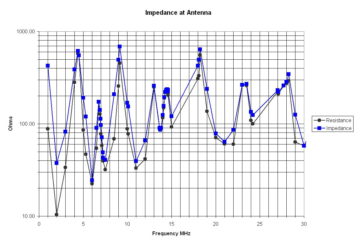
Figure
8. Calculated Impedance at Load |
|---|---|
 |
 |
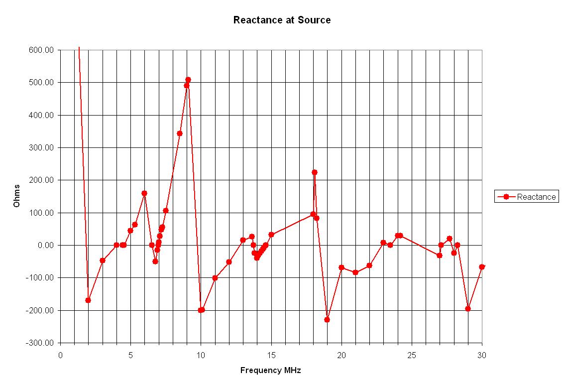
| Figure
9. Measured Reactance at Source |
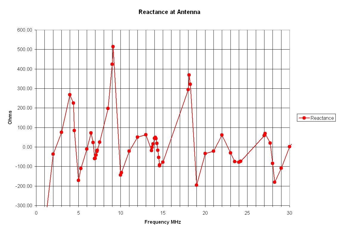
Figure
10. Calculated Reactance at Load |
 |
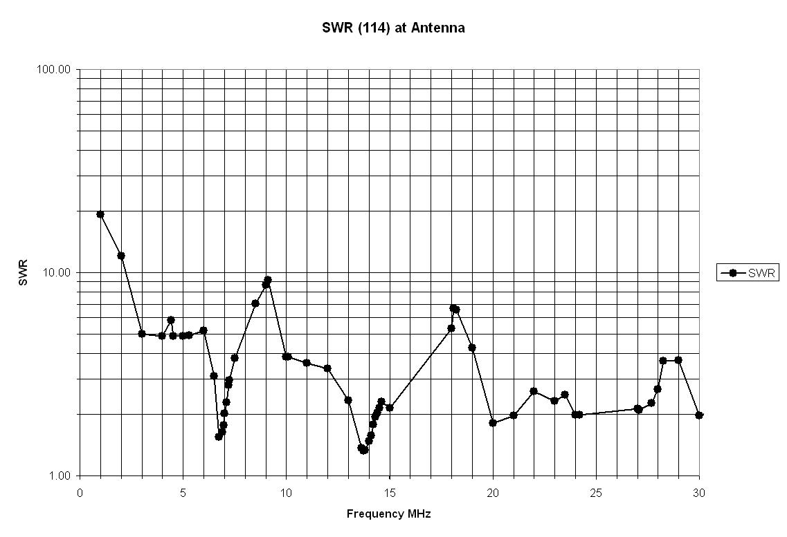 |
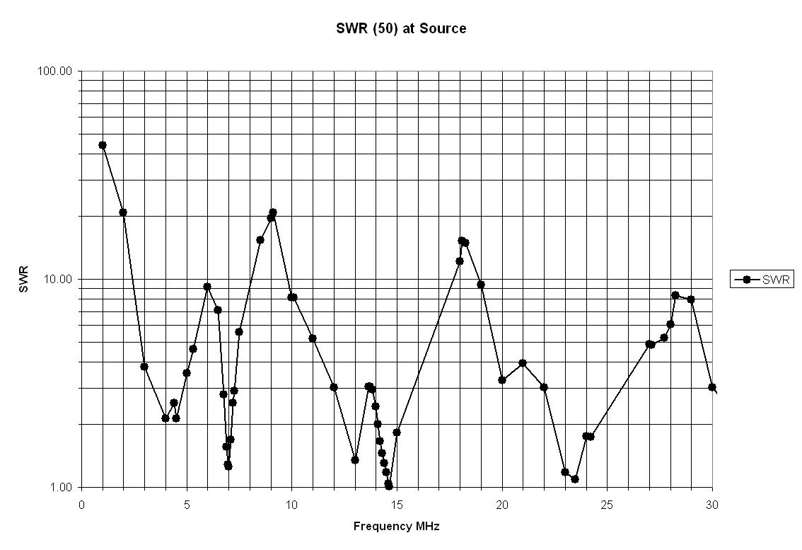
| Figure
11. Measured SWR at Source |
Figure
12. Calculated SWR at Load |
 |
 |
 |
| Figure
13. Characteristic impedance Z0 vs.
frequency |
Figure 14. Velocity
factor vs. frequency |
Figure
15. Attenuation vs. frequency |
|---|
 |
| Figure 16. Transmission Line Details program antenna system calculations |
|---|