AN-SOF simulation of a 10m free space dipole
10 Meter Vertically Oriented Free Space Half-Wave Dipole
This is a quick walk through on how to simulate a 10 meter dipole using AN-SOF software. Get your trial AN-SOF Software at: https://antennasimulator.com
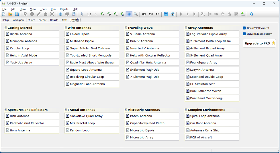
Starting up AN-SOF yields the following window, allowing selection of example analysis / walk-through document. Users can select File / New to start a new, from-scratch simulation.
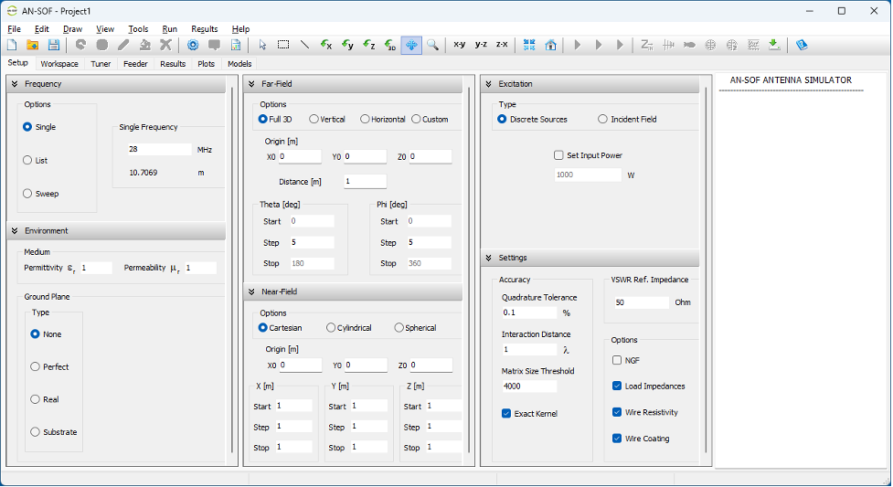
Select File / New and a new model window appears. Next select the Setup tab in the working area window. Check each of the window frames and set to match up with the values/selections below to enable simulation of our 10m half-wave center-fed dipole.
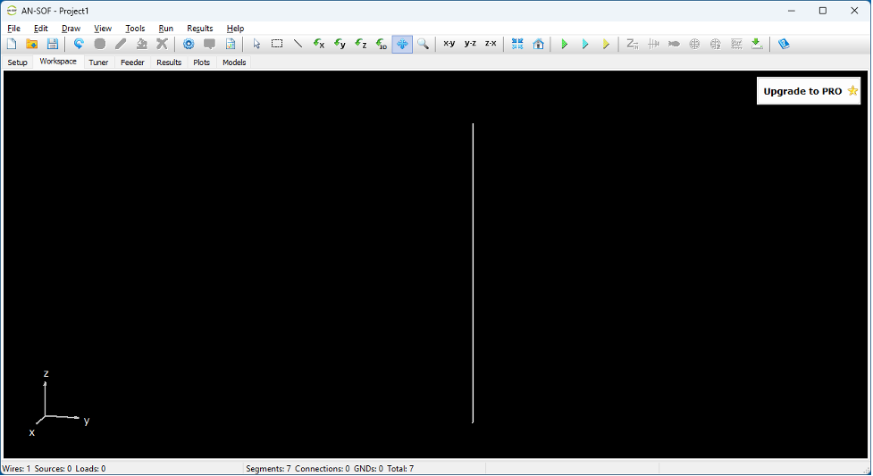
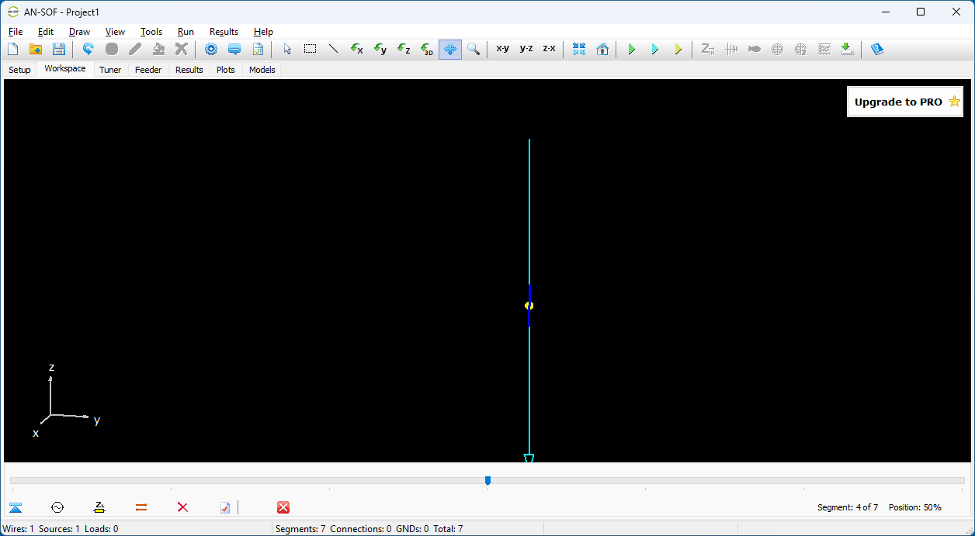
Click on the Workspace window tab. This where the wire antenna model will be created.
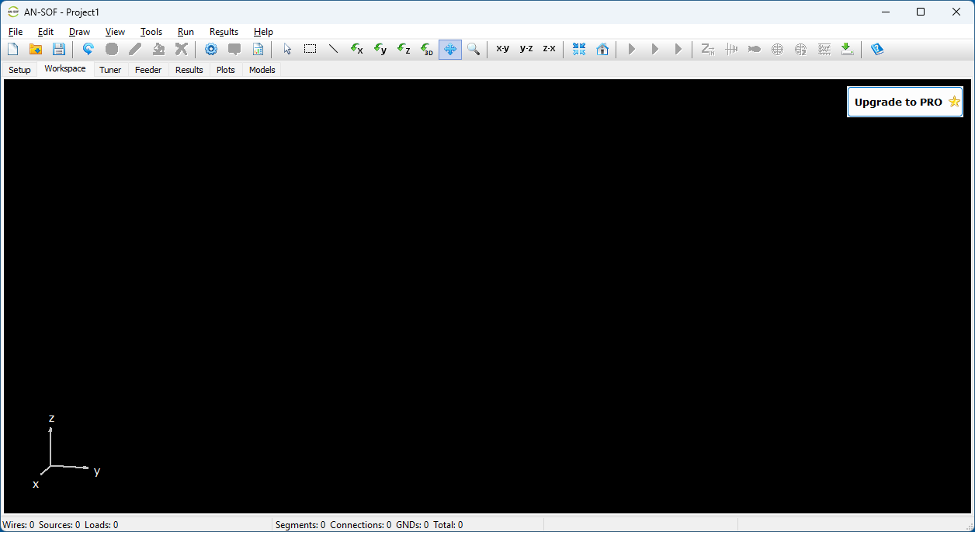
Right-click on the black window and a pop-up appears, left click on Line, a new sub-window appears.
On the Line tab, enter Z1 = +3, Z2 = -3
Click on Attributes tab, enter Number of Segments = 7 (odd number for a dipole, yields ability to put the feed point on the center segment, i.e., 50%).
Set Cross Section (wire radius = 5 mm).
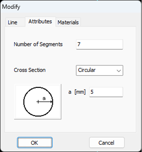
Click on OK to create the 7 segment wire.
Right-click on the wire just created and select the top menu item Source / Load / …
A new sub-screen appears at the bottom of the window. Move the blue slider bar until the blue pointer is in the middle (Position = 50% appears at right edge). Note that the blue segment in the antenna wire moves from one end to the middle segment.
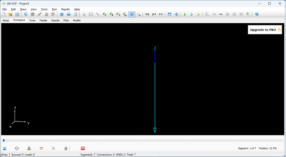
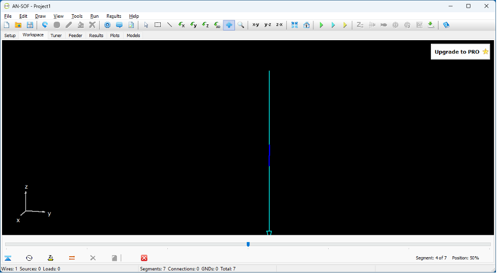
Click on the second icon in the new sub-window (looks like an AC source circle). A new window pops up to set the source (feed point) parameters.
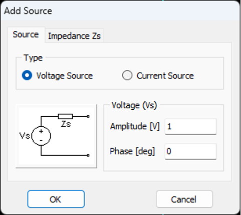
Click on the OK button to select source and place in center location. A yellow circle appears in the middle of the wire. A similar process would be used to create an off-center-fed-dipole (OCFD), setting the feed point to the desired position along the wire for that antenna version. The number of segments may be increased to yield better feed point location fidelity. Note that the free (unlimited trial) SW version has a limitation on the number of segments in your model.
Roll the mouse middle wheel up and down, and note that the size of the line changes accordingly. You can’t move the line up/down or left/right as there is nothing to move it against in this simple free space model. (See next example vertical-over-ground to see how moving the model in the workspace can be accomplished.)
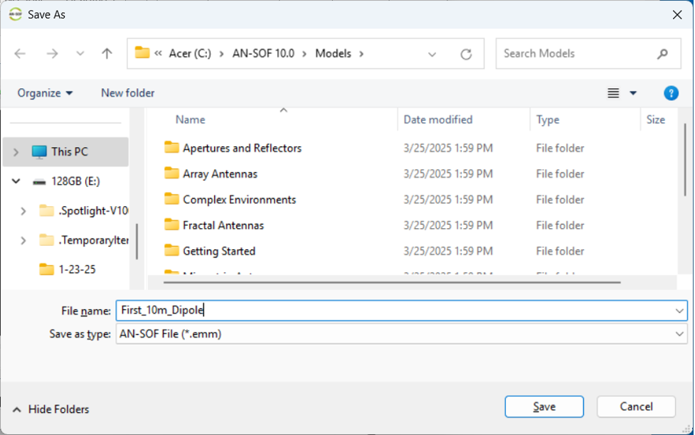
Save your work (File / Save-As / new-window-appears-name-file-and-save).
Use the top level Run menu to “Run-ALL”. A new window appears and the process steps are completed quickly.
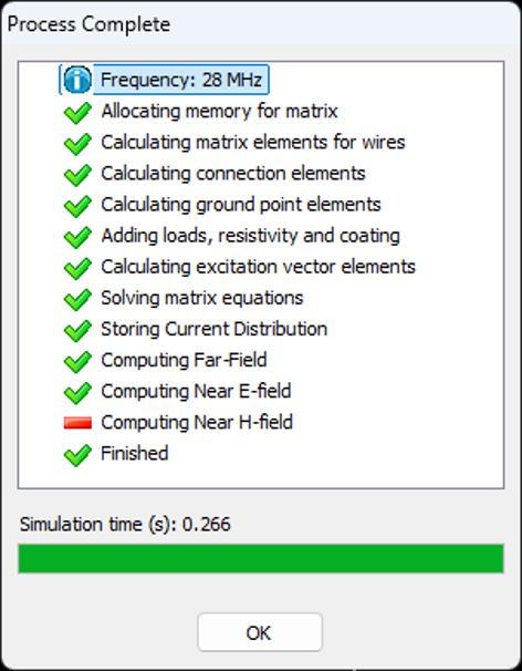
Click OK button and click on top level Results menu.
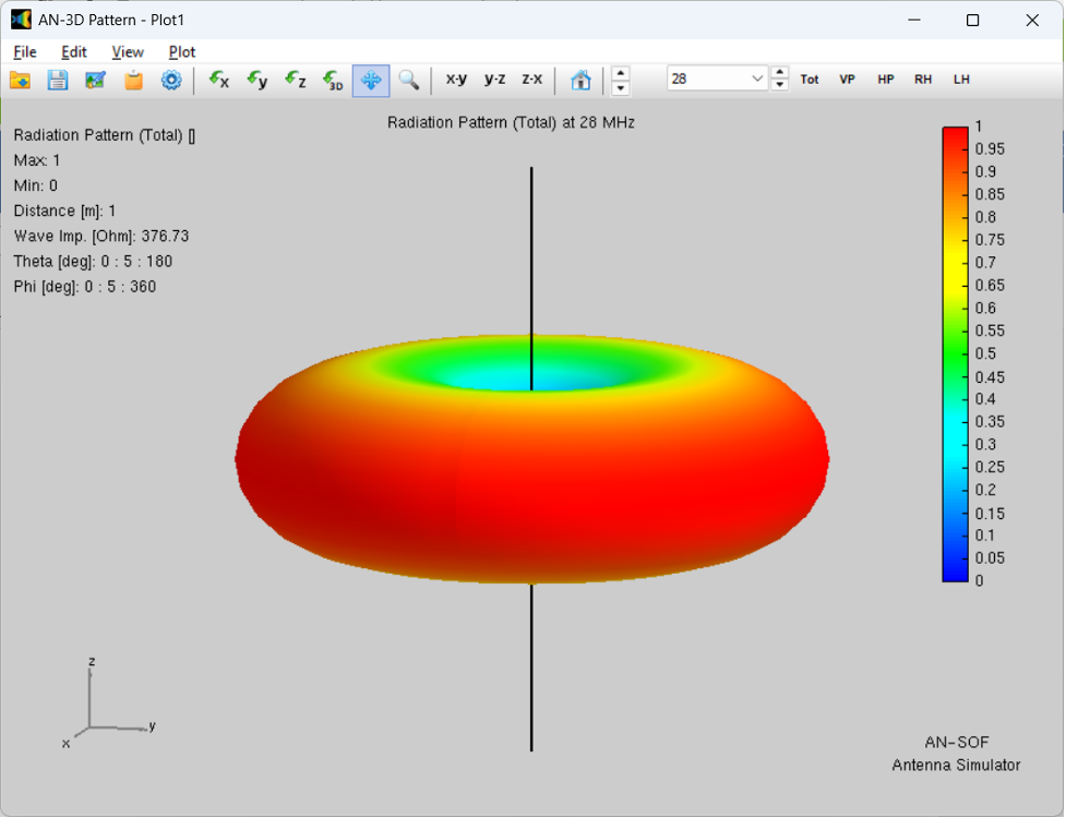
Select Plot Far-Field Pattern > 3D Plot.
A new plot window appears.
There are axis rotation selections (green curved arrow next to axis name) that allow examining the plot from different angles. You can save the plot using the menu selections along the top two rows.
A cut into the above pattern can be obtained by selecting the top level Results menu, then selecting Plot Far-Field Pattern drop down, then selecting Polar Plot 1 Slice. A pop up window appears titled Radiation Pattern Cut. Select radio button Fixed phi, then click OK to yield a cross section of the pattern as follows:
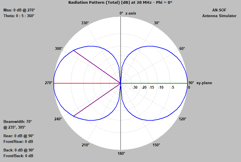
Note that the vertical (3 dB) beamwidth is 70 degrees.
Analysis Summary: This plot shows the expected donut-shaped far field radiation pattern of a vertically oriented free space 28 MHz (10m) dipole. We used a 6 meter long, 10 mm diameter wire for our element, with center feed used for the simulation.
Congratulations, you have completed your first antenna simulation. Lots of fun and learning are ahead!
For next-steps, see the next posting for tuning the 10m free-space dipole.
Here is the main page for my AN-SOF antenna simulations.